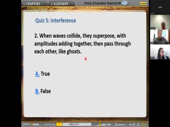
| 00:00 | We will, we will, so will begin this afternoon with addressing the |
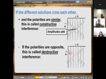
|
| 00:07 | that you emailed uh to me uh the last time I saw you and |
|
| 00:14 | uh if you didn't email me then it right now. So let us |
|
| 00:21 | check my email. OK. So one from Carlos. Wow. So |
|
| 00:44 | is AAA really good question. And um so Utah left, uh So |
|
| 00:52 | me uh recover the zoom session. uh folks can uh can, can |
|
| 00:57 | hear me, give me a thumbs , Carlos, can you hear |
|
| 01:01 | OK. So Carlos asked under what can we consider that the R MS |
|
| 01:08 | is equal to the NMO velocity? . So that's a really good |
|
| 01:13 | So we just derived the, the out velocity. Uh uh uh |
|
| 01:20 | and so we'll, we'll shortly see to correct for the move out velocity |
|
| 01:26 | a lot of assumptions, right? what, what were those assumptions? |
|
| 01:29 | the, the assumptions were that the was flat layers. And furthermore, |
|
| 01:35 | was uh an unstated implication that they be co flat layers. That is |
|
| 01:42 | layers should be um um uh uh thin layers, what are thin |
|
| 01:49 | thin layers are thin compared to the wavelength. So of course, we |
|
| 01:53 | lots of seismic wavelengths uh uh in the seismic signal, right, we |
|
| 01:57 | all a whole spectrum of frequencies and have a whole spectrum of wavelengths. |
|
| 02:02 | but uh some of them uh are energetic than others, some of them |
|
| 02:08 | more power at, at that frequency others. And so what we say |
|
| 02:13 | is that consider the dominant wavelength, sort of corresponds to the dominant uh |
|
| 02:20 | , which you can see and on workstation with the, the uh the |
|
| 02:26 | extent of the arrival. So if arrival is uh uh uh uh you |
|
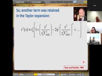
| 02:30 | , a pulse of, of energy with uh uh over about uh 50 |
|
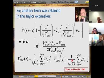
| 02:36 | , then we can sort of consider the dominant frequency even without doing a |
|
| 02:43 | year analysis. And then there will a corresponding um uh uh a corresponding |
|
| 02:49 | wavelength uh to that. And the corresponding to that frequency depends on the |
|
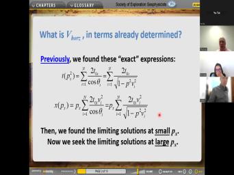
| 02:56 | velocity, of course, but you sort of make an estimate. Uh |
|
| 03:01 | And uh so, uh uh it turns out that the dominant wavelengths in |
|
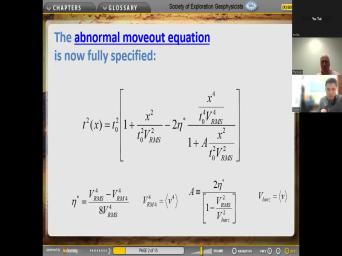
| 03:07 | signals coming from reservoirs, you a few 1000 ft down uh that |
|
| 03:14 | uh wavelength is a couple of 100 long. So normally, uh the |
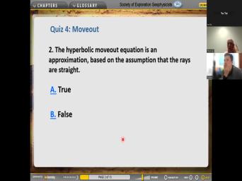
|
| 03:22 | are a lot thinner than that. , right there, you have an |
|
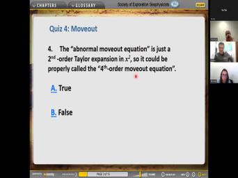
| 03:25 | of an assumption that we made as were deriving the dick's relationship for |
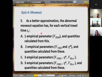
|
| 03:32 | uh so, uh for the R velocity, uh and for the move |
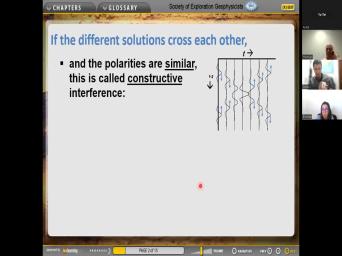
|
| 03:40 | , uh uh uh that's AAA an where uh we made an assumption which |
|
| 03:46 | obviously wrong in our experience. the beds are a lot thinner than |
|
| 03:53 | . And so, uh uh what did we assume? Well, we |
|
| 03:56 | that the individual course beds were And so that's probably not true |
|
| 04:04 | So these are bo uh both instances the R MS velocity is not equal |
|
| 04:10 | the NMO velocity. Remember the NMO , we are going to determine empirically |
|
| 04:16 | our um workstations by uh uh by c by testing a lot of different |
|
| 04:23 | and choosing that, that, that of which flattens the gathers, which |
|
| 04:28 | corrects for the move out for uh for the gathers in the data. |
|
| 04:36 | gonna talk more about that process but that's enough for now. So |
|
| 04:41 | see that the move out velocity is empirically determined thing or as the R |
|
| 04:46 | velocity is a property of the it's, it uh we calculated it |
|
| 04:52 | a function of the um uh layer and the local velocities uh everywhere in |
|
| 05:00 | over birth. So that's sort of property of the subsurface. And uh |
|
| 05:06 | um uh we will be addressing um shortly uh issues that arise when we |
|
| 05:14 | the difference between R MS velocity and velocity. But uh uh uh that's |
|
| 05:23 | very good uh question, Carlos and uh that sort of thing is gonna |
|
| 05:29 | up time and time and again. , what I'm gonna do right now |
|
| 05:35 | uh let's see, I don't think shared my screen have. I, |
|
| 05:38 | don't think I've shared my screen with . OK. So, uh we |
|
| 05:42 | need to share the screen uh Let me go back and see what |
|
| 05:46 | questions we have. Here's one from uh le le and she says uh |
|
| 05:52 | uh on slide 61. Why is curl free part used to derive the |
|
| 05:59 | wave and the divergence free part is sheer wave. OK. So let's |
|
| 06:05 | uh uh uh let's go back to slide. So what I'm gonna do |
|
| 06:12 | get out of the email remembering that gonna do slide 61. Oh What |
|
| 06:29 | an elasticity. Yes. Yes. oh OK. Any, any |
|
| 06:35 | OK. So, uh uh before do that, I am going to |
|
| 06:41 | up that slide from elasticity and its on a second. Here we |
|
| 06:58 | Um All right, here we got elasticity. OK. So uh now |
|
| 07:13 | a good time to share the And so here we go, share |
|
| 07:18 | screen and this is what I'm gonna . OK. So everybody can see |
|
| 07:25 | screen now. And yes. Uh this beginning slide of that. So |
|
| 07:32 | me just go down to slide 62. Mm 62. I don't |
|
| 07:42 | that's the right one. Oh So I think it's a wave |
|
| 07:51 | Yes. OK. So uh I'm stop sharing this file and go back |
|
| 07:59 | uh the powerpoint oops powerpoint and uh get out of this and find a |
|
| 08:10 | equation would be extra three. Here go. And now I'm gonna |
|
| 08:23 | OK. She uh share the OK. So here is now um |
|
| 08:35 | lecture three. OK. So now looking for slide 61. Uh Is |
|
| 08:52 | the one? OK. So um , uh sure I ask, |
|
| 09:01 | I think everybody can see this. . Yeah, everybody can see |
|
| 09:06 | So, um uh now, so uh start at the beginning. Uh |
|
| 09:14 | had an equation. We have uh uh uh let me just back up |
|
| 09:19 | slide. OK. So if the medium is uniform, we have the |
|
| 09:28 | equation. Uh can everybody see my here? OK. So uh that |
|
| 09:35 | uh uh everything is in there that all uh uh uh uh this is |
|
| 09:41 | , the particle displacement and that's uh particle displacement resulting from all arrivals depend |
|
| 09:49 | uh uh uh direct arrivals, reflected . Uh um uh ground roll, |
|
| 09:56 | is in there. OK. So uh uh key waves and she |
|
| 10:02 | everything is in there. So so the next step we're uh we're |
|
| 10:06 | go to uh uh uh uh the by uh uh Mr Helmholz German physicist |
|
| 10:16 | in the 19th century. And uh , he proved to us that for |
|
| 10:23 | we have um uh a vector quantity the displacement, which is defined everywhere |
|
| 10:31 | space and time, then we can divide that into a part which has |
|
| 10:37 | curl and a part that has zero . So we call this the curl |
|
| 10:42 | part and the divergence free part. so, uh now the question, |
|
| 10:47 | , what uh uh Lily is asking why do we call this thing |
|
| 10:52 | the curl free part, why do call that the P wave part? |
|
| 10:57 | the, the reason is that uh that's sort of a, I think |
|
| 11:00 | a pretty good English description of the A P wave goes through uh a |
|
| 11:08 | as it goes through, it's squeezing rock back and forth. It's not |
|
| 11:12 | the rock at all. So that's we say it's curl free. Maybe |
|
| 11:16 | should have said twist free. But mathematicians have the word curl for uh |
|
| 11:23 | a particular operation um um of, vector calculus. Uh So, uh |
|
| 11:31 | a, a certain combination of derivative we're, we're gonna go back and |
|
| 11:37 | that in a second. And uh it's a pretty good English word |
|
| 11:41 | say that uh that uh that, combination of uh of uh derivatives uh |
|
| 11:51 | that uh the uh the, the field like displacement has zero curl. |
|
| 12:00 | in the same way, the other has zero divergence. And uh when |
|
| 12:04 | think about as a sheer wave goes a rock, it's twisting the rock |
|
| 12:09 | it's not uh uh squeezing it and unsqueeze it. So it has |
|
| 12:13 | convergence and it has no divergence. . So the divergence uh part is |
|
| 12:19 | uh is a part where the divergence this part here is zero. So |
|
| 12:25 | re uh let's uh review uh shortly we mean by the curl of a |
|
| 12:32 | field and the divergence of a vector . OK. So, uh I |
|
| 12:38 | these are good English names, you , taken from the German names. |
|
| 12:42 | are good uh uh English names for the portions of this total displacement field |
|
| 12:49 | are due to P waves and to waves. OK. So now I'm |
|
| 12:53 | go back uh uh I'm gonna go uh back here. Uh So I |
|
| 13:05 | uh you, I, I think not sharing anything now. Is that |
|
| 13:10 | ? Yeah. Not, not sharing now. So I'm going to uh |
|
| 13:14 | to the powerpoint and I'm gonna find ? Yeah. OK. So now |
|
| 13:30 | gonna share again, I share my again. And so OK. So |
|
| 13:45 | think you can see this now, is the entry screen for the math |
|
| 13:50 | F. So let's find in Uh Let's see. Uh So this |
|
| 13:57 | the, the fourth topic is uh calculus. So I'm going to find |
|
| 14:04 | in the file. And uh so can see right here, that's the |
|
| 14:09 | topic and that it would all get calculus right here. OK. So |
|
| 14:20 | , let's uh see. So we uh uh uh oh, good, |
|
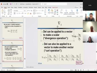
| 14:27 | . Thank you your time. Just second here. OK. We define |
|
| 14:41 | vector and it's a vector operator and has uh uh three components of 12 |
|
| 14:49 | three. And each component is this derivative with a corresponding partial derivative with |
|
| 14:56 | to X of I. And so vector looks kind of funny, isn't |
|
| 15:01 | ? And it has no meaning. when it uh when it operates on |
|
| 15:06 | vector, uh uh then it has meeting. So we're gonna go to |
|
| 15:10 | next slide. OK. So this the second slide in this uh uh |
|
| 15:19 | . So if this vector operator del this delt, if it's applied, |
|
| 15:25 | it operates on a scalar, then uh uh uh uh the resulting quantity |
|
| 15:33 | called the gradient and that's a So you can see here that this |
|
| 15:39 | we just defined back here, you verify this for yourself. So uh |
|
| 15:44 | operate uh that on a scale, got three components. Each one of |
|
| 15:48 | is uh uh uh a partial derivative respect to the corresponding uh position |
|
| 15:57 | And we have five is in. that's, this is a spelling out |
|
| 16:03 | this means Dell operating on five. . No, it also says that |
|
| 16:12 | can be applied to a vector and uh Adele applies to a vector. |
|
| 16:17 | so you see that same operator partial spec X I uh uh operating uh |
|
| 16:24 | this vector U I. And now see that the I is repeated, |
|
| 16:28 | uh it's uh twice. So this , this is a sum I equals |
|
| 16:33 | to 3 du ID X one plus I uh uh du two D uh |
|
| 16:41 | two, et cetera. And of , you see how that's different back |
|
| 16:45 | , we made a vector. And uh uh Ooo over here, we're |
|
| 16:52 | um uh a scaler by summing up three derivatives. And how did that |
|
| 16:58 | ? Because we're operating with Dell on vector. Whereas back here we operated |
|
| 17:04 | Dell on a Scaler. OK. , there's another way that Dell can |
|
| 17:11 | on a vector. And here is uh that other uh way this is |
|
| 17:18 | the curl operation. So we have cross U makes a vector. And |
|
| 17:24 | are the definitions of the vector. you see that's a lot more complicated |
|
| 17:29 | this one. And let me see , what do we have next? |
|
| 17:34 | , next to you uh uh uh goes on to. So this is |
|
| 17:40 | for now that we can uh uh this is the operation of uh of |
|
| 17:46 | and uh going back to Helmholtz, that Helmholtz said that there was, |
|
| 17:51 | was a uh uh any vector field can be divided into a part, |
|
| 17:57 | part where divergence of U is zero another part curl of U is |
|
| 18:03 | And so the, and the part is divergence of 0 to 0, |
|
| 18:07 | the uh uh the shear wave and uh part with the curl is zero |
|
| 18:14 | the P wave. So does that your question? Really of? |
|
| 18:21 | So that's sort of a review And, and uh so um let |
|
| 18:28 | uh get out of this and go to uh the email. OK. |
|
| 18:44 | . So here's another question from le slide 114. Does the reciprocity of |
|
| 18:51 | of elasticity have the condition that the is elastic? Um OK. Uh |
|
| 19:01 | So then she's got some more These are really good questions, |
|
| 19:04 | OK. So uh can everybody see ? I don't think so. |
|
| 19:12 | No. Yeah, no, nobody can see it. So hold |
|
| 19:15 | . Uh I, I share this for there were money. OK. |
|
| 19:25 | this is my email inbox and this um uh from a late, so |
|
| 19:31 | talking about the slide 114. I this is um uh I forgot which |
|
| 19:39 | uh I think this is the E election. So she says, does |
|
| 19:44 | reciprocity theorem of elasticity have the condition the medium is elastic. And of |
|
| 19:50 | , that the answer is yes. uh When we uh we didn't derive |
|
| 19:55 | uh uh theorem of elastic, the theorem. But um because it has |
|
| 20:01 | name elasticity in there, the, answer to this question is yes. |
|
| 20:05 | uh But now here comes the really question actually are all the rock property |
|
| 20:12 | elastic. OK. So the answer that is no, in fact, |
|
| 20:20 | of the rocks in the subsurface are , none of them. Why is |
|
| 20:27 | ? Because Mr Hook in the 17th defined elasticity for homogeneous materials, you |
|
| 20:35 | , like uh uh copper and like and like iron and rocks are not |
|
| 20:43 | that, right? Uh rocks are rocks have grains and pores and who |
|
| 20:48 | what else. And uh uh so its face, none of the rocks |
|
| 20:54 | the subsurface are elastic. What a . So you should be asking yourself |
|
| 21:01 | then are we studying elasticity? And know that all of your professors and |
|
| 21:07 | of your previous courses assume that the of the, of the uh subservient |
|
| 21:13 | elastic. Well, so uh Mr would have been mystified. He would |
|
| 21:19 | said, well, uh uh uh they're not elastic, they are |
|
| 21:24 | , they have grains and they got and then the pores may be |
|
| 21:28 | maybe oil, maybe liquid and the are gonna have a different pressure on |
|
| 21:32 | than the grains, right? And grains are gonna be different kinds of |
|
| 21:37 | . There's gonna be grains of quartz grains of, of calcite and everything |
|
| 21:41 | . Everything is heterogeneous on the grain on a rock. So Hook would |
|
| 21:48 | said, well, no, of not that my theory doesn't apply |
|
| 21:52 | Ok. So we are going to those issues later in the course. |
|
| 21:59 | we're gonna find out that everything we about elasticity is gonna be replaced by |
|
| 22:06 | more complete theory due to a guy Beau starting in 1941. And he |
|
| 22:16 | about all the complications that arise because are heterogeneous, lots of complications. |
|
| 22:26 | , here's the good news uh uh in uh um in a certain approximation |
|
| 22:32 | we'll get to at that time, uh the results of coral elasticity are |
|
| 22:40 | same as the results of elasticity only certain small changes. You know, |
|
| 22:48 | example, we're gonna find out that later in the lecture, we're gonna |
|
| 22:52 | later in the course, we're gonna out that according to the uh uh |
|
| 22:58 | the theory of chal eas, uh rocks have uh properties which depend upon |
|
| 23:07 | average composition of the rock. Uh But here's a complication. It |
|
| 23:13 | not only on the average um position also on the details of the micro |
|
| 23:21 | . So it makes a difference. example, if um uh if the |
|
| 23:26 | are round or if the pores are , same porosity, you can imagine |
|
| 23:32 | case where uh uh different kinds of different uh details of micro geometry. |
|
| 23:41 | so beau explained to us that under circumstances, the properties of the rock |
|
| 23:50 | be uh uh defined uh using the of elasticity. But recognizing that the |
|
| 23:57 | are heterogeneous and we gotta be talking average composition and uh average uh micro |
|
| 24:06 | uh you know, a a and average pressure, just think about |
|
| 24:10 | Uh uh you know that uh uh , you know that the rocks in |
|
| 24:19 | subsurface are not, are under high , but most of the pressure from |
|
| 24:23 | overburden is carried by their brains and uh pressure in the fluids is |
|
| 24:34 | maybe a lot less or maybe only little bit less. So that's a |
|
| 24:38 | issue for us in the oil and business is to deal with the fact |
|
| 24:43 | I subsurface pore pressure. Yeah. those are all advanced topics which we |
|
| 24:50 | not gonna concern ourselves with. uh we are learning about elasticity knowing |
|
| 24:58 | we made all kinds of, of approximations which are obviously not true and |
|
| 25:05 | smart to be questioning those. I'm you're questioning those. Uh uh But |
|
| 25:11 | uh because you're here at the University Houston, we are gonna go on |
|
| 25:16 | teach you about some of the uh realistic assumptions that is by the end |
|
| 25:23 | this course, we will have um on a lot of, of the |
|
| 25:30 | of the sim simplifications that we're uh, right now. So, |
|
| 25:34 | now I'm teaching you something which, , uh uh Robert Hook would not |
|
| 25:39 | surprised to see what I'm teaching her about uh uh uh divergence free and |
|
| 25:45 | free and so on. Uh um uh those ideas came from Helmholz |
|
| 25:52 | lived, uh hundreds of years after . But the Foot Corp listening in |
|
| 25:57 | lecture, if he were uh listening Zoom, he would have said |
|
| 26:01 | Yeah. II, I believe that came along after I died. That |
|
| 26:05 | hum. And he showed that and , that probably makes sense. He |
|
| 26:10 | book would probably be thinking, I'd like to see a proof but |
|
| 26:13 | , he could see that uh that makes sense and he would be |
|
| 26:18 | he would be 100% with the program till now. OK. Now you |
|
| 26:24 | another question. If one side has gas reservoir or, or there is |
|
| 26:31 | isotropy exiting. Does the reciprocity theorem ? OK. So um now I'm |
|
| 26:38 | sure what you mean here. You one side or one side of what |
|
| 26:52 | uh you, you need to speak a lot more loudly. That is |
|
| 26:58 | we have OK. What's on the side? The seal side? And |
|
| 27:04 | ? OK. So uh uh so you all uh uh di in what |
|
| 27:10 | uh is uh asking now is a case where we have a reflection off |
|
| 27:17 | uh the top of a reservoir and one side, there's a gas and |
|
| 27:22 | uh maybe anisotropy on the other OK. So now these questions are |
|
| 27:29 | because you're um you're talking about uh sides, right? You're talking uh |
|
| 27:34 | the reciprocity theorem only applies to a body, right? So, and |
|
| 27:40 | re reciprocity there, there's no one , there's no the other side. |
|
| 27:45 | I can tell you that the reciprocity applies if that single uniform body is |
|
| 27:54 | . Yeah, we, we the, the reciprocity theorem does not |
|
| 27:59 | uh isotropy and it, it doesn't P waves or sheer waves anything. |
|
| 28:05 | uh suppose uh uh uh uh uh inside a body uh uh uh remember |
|
| 28:12 | ellipse that we had where we talked the rest of the price. So |
|
| 28:16 | inside that body um uh uh where it bounced off of the inside of |
|
| 28:22 | , of the uh ellipse that some it got converted to shear waves, |
|
| 28:27 | know, that happens at a, , in reflection P wave hits on |
|
| 28:32 | uh um uh interface and uh uh of the reflected energy uh is turned |
|
| 28:40 | she waves. So uh uh that's , that kind of mode conversion is |
|
| 28:47 | in the um um um and the it there. And uh so uh |
|
| 28:59 | why I told you the reciprocity theorem is very deep there and uh uh |
|
| 29:05 | hardly any limitations to it. And , when that uh um when, |
|
| 29:15 | that uh puzzle was posed in the , it was now 30 years |
|
| 29:21 | Uh It caused a lot of it caused a lot of discussion and |
|
| 29:26 | lot of people uh uh uh uh more uh were educated during, by |
|
| 29:33 | discussion because uh the theorem uh uh hardly any limiting assumptions to it. |
|
| 29:41 | , the main, the main limiting is that it's uh elastic, like |
|
| 29:46 | said, a on the first. the rest of process works for |
|
| 29:54 | OK. Now, II I, think we didn't, we didn't talk |
|
| 30:01 | this before, but the reciprocity thera a, is more complicated than you |
|
| 30:12 | know. Uh If you, if if you're thinking that the reciprocity there |
|
| 30:18 | the following interchange source and receiver and get the same signal that's a special |
|
| 30:26 | . And so uh we will talk about the rest of the later. |
|
| 30:32 | . So thanks for those questions. now I'm gonna scroll down here. |
|
| 30:43 | a question from um I'm saying that says, I hope I can answer |
|
| 30:51 | myself these questions before Friday and we'll new and different questions by Friday. |
|
| 30:58 | . OK. Now, look at , uh she has the same question |
|
| 31:02 | uh that Lee Lee had, I I did not do a very good |
|
| 31:07 | of uh of uh of uh explaining point for. So that's why I |
|
| 31:13 | like to come back. Uh the day and talk about it. |
|
| 31:18 | Uh So uh uh uh Rosa, you, are you happy with |
|
| 31:22 | Uh uh question now? Yes, , I am. Thank you. |
|
| 31:27 | question she says is for migrating the is the ray pa equation more convenient |
|
| 31:32 | use than the wave equation. So the answer to that depends upon the |
|
| 31:38 | the uh the migration algorithm that we . And so um uh uh when |
|
| 31:46 | left uh uh as you know, used to work for Amaco and then |
|
| 31:51 | BP. And I retired many years when I left BP in 2000 and |
|
| 32:00 | and six, I left BP and retired in 2006. And I, |
|
| 32:05 | that time, I calculated in I looked around inside BP. At |
|
| 32:11 | time, we had 26 different uh to do migration, 26 different |
|
| 32:19 | And I'm sure they have more now some of them, they use more |
|
| 32:23 | others. Some of them are obsolete . But uh all of these uh |
|
| 32:28 | uh uh uh all, all these made different assumptions and uh you |
|
| 32:34 | some of them uh uh were good for uh one dimensional bodies and others |
|
| 32:40 | for three dimensional bodies and so Some were in it or low frequency |
|
| 32:44 | some are high frequency. So some them were K Kirk off migration and |
|
| 32:49 | of them were reverse time migration. you see all the different flavors of |
|
| 32:55 | which are out there. And I'm gonna go into these in any detail |
|
| 33:00 | all. In this course, you another course uh coming up uh in |
|
| 33:04 | few weeks to talk about uh uh with data. And uh that uh |
|
| 33:11 | will tell you about these. I it's Professor Hill, I think it's |
|
| 33:15 | Hill. Is that correct? So he is a real expert in |
|
| 33:23 | things. And so he will tell uh better than me. OK. |
|
| 33:30 | then uh let me stop sharing this I go back to uh so you |
|
| 33:40 | to back to where we were when left off on Saturday? OK. |
|
| 33:53 | I'm gonna uh share that. So this is where we ended up |
|
| 34:13 | uh uh with the uh the dix which is right here. Um And |
|
| 34:20 | also call this the Hyperbolic Moveon Oh I, and I want |
|
| 34:25 | I want to start, OK. I, I think um you say |
|
| 34:39 | need to, I need to uh . OK. So I'm gonna stop |
|
| 34:45 | and I'm gonna start sharing suspension. ? One still sharing screen one. |
|
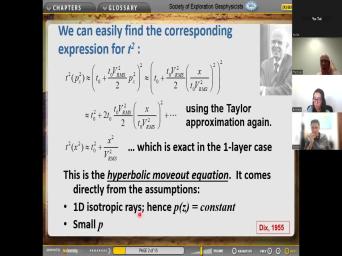
| 35:06 | Swimming through it. OK. uh uh these are the assumptions that |
|
| 35:20 | made uh that uh Dick made ma many years ago, many years |
|
| 35:26 | you can see there in the lower hand corner and he did this a |
|
| 35:33 | time ago. You can imagine that had computers in that time, which |
|
| 35:38 | hardly anything compared to what we have . As a matter of fact, |
|
| 35:42 | don't think he had any, any whatsoever back in 1959 55. So |
|
| 35:48 | , he was doing this with paper pencil and he was expecting that, |
|
| 35:53 | , people would be implementing this with and pencil. Well, we can |
|
| 35:58 | a lot better these days, of . Uh, But uh we're still |
|
| 36:01 | uh keeping these assumptions that uh uh a one dimensional uh subsurface, you |
|
| 36:10 | , not true isotropic, not Um A small ray parameter. P |
|
| 36:18 | , uh uh so uh that is for short offsets, but for long |
|
| 36:22 | offsets, that's not true anymore. uh uh uh these are limitations on |
|
| 36:31 | formula uh which we are gonna uh upon in the next few minutes. |
|
| 36:40 | . So, uh of course, we, if we did have um |
|
| 36:45 | uh if we did have a uniform uh one D body like we assumed |
|
| 36:51 | , and if it had AAA velocity this, we would get the same |
|
| 36:58 | . Yeah. In fact, the the subs are more complicated than |
|
| 37:04 | Now, I um uh uh we up last time with uh I I |
|
| 37:13 | on this slide here where we said , we're still gonna be able to |
|
| 37:19 | uh this formula, the hyperbolic move equation uh uh even for the case |
|
| 37:24 | dipping layers and anisotropic layers, if regard the move out velocity to be |
|
| 37:31 | processing parameter with, which would be by looking at the data itself. |
|
| 37:36 | when we do that, we're gonna that normally, uh these two are |
|
| 37:40 | equal to each other. That was Carlo's question was um uh beginning. |
|
| 37:49 | , uh uh nonetheless, let us I keep that in the back of |
|
| 37:55 | mind that the about velocity is gonna probably gonna be different than the R |
|
| 38:02 | velocity. But carry on with the that Dick gave back in 1955 |
|
| 38:08 | that was almost three quarters of a ago. That's a long time |
|
| 38:14 | And we're still using it today. this is what he thought, he |
|
| 38:20 | , uh empirically, we find out the move out velocity varies with |
|
| 38:25 | And so, uh you know, there's lots of, lots of reflections |
|
| 38:29 | lots of layers. And so here's definition of the R MS velocity at |
|
| 38:34 | bottom of the nth layer. So see we got AAA sum over layers |
|
| 38:40 | equals one to end of uh two the one way travel time. So |
|
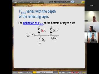
| 38:46 | the two way travel time times the uh square in the square of the |
|
| 38:51 | velocity. And then we're dividing by uh so these are like weights, |
|
| 38:58 | the two way travel time is the for the um for this Irish. |
|
| 39:08 | I wanna make sure that you are my use of the English word |
|
| 39:13 | Uh, that means that uh, turn in this average has a, |
|
| 39:21 | a, a weighting of this And down here the sum of the |
|
| 39:25 | so we can repress the sum of weights as a total travel time. |
|
| 39:31 | that's the definition at the bottom of nth layer. So the, |
|
| 39:37 | the bottom of the overlying layer looks same way except it's got uh uh |
|
| 39:42 | got the sum only goes up to minus one. And the bottom here |
|
| 39:47 | the, is the to travel time to the bottom of the overlying |
|
| 39:56 | So then just by um uh uh by manipulating those two equations, we |
|
| 40:06 | find the uh the uh the, interval velocity IV I in that nth |
|
| 40:14 | . So uh this is the formula we had for uh the bars velocity |
|
| 40:20 | the bottom of the nth layer that out the, the top term leaving |
|
| 40:26 | other N minus one terms here. what we're doing here. And uh |
|
| 40:35 | so this quantity here from the previous is given by this time parameter, |
|
| 40:43 | way travel time to the bottom of up overlying layer times the R MS |
|
| 40:51 | down to the overlying layer. And you dissolve for the N solve for |
|
| 40:57 | parameter here, and uh B we the velocity in that nth layer. |
|
| 41:02 | see it, it's uh uh it's to the uh uh the travel time |
|
| 41:08 | the bottom of the nth layer times R MS velocity at that bottom of |
|
| 41:14 | layer minus the corresponding from overlying layer by uh uh uh run by |
|
| 41:27 | yeah, divided by uh by a total time plan. And so we |
|
| 41:32 | call this dick differentiation and this was course uh derived by dick a |
|
| 41:39 | long time ago. Now, why we want to do this? It's |
|
| 41:47 | we want to know all of those velocities so that we can find the |
|
| 41:53 | depth. So we know the travel uh directly from our workstation. And |
|
| 41:59 | we know the local velocities in each . So we can just add them |
|
| 42:03 | and find the depth. But think this, remember the question that Carlos |
|
| 42:18 | , he said, what happens if is not equal to VR MS, |
|
| 42:24 | the previous calculation to determine these these local velocity that would be |
|
| 42:30 | And so we would get uh we calculate the wrong depth. So we |
|
| 42:36 | call this a time depth miss And it's very common, very common |
|
| 42:44 | uh uh processing data, you calculate in this way uh or uh an |
|
| 42:52 | way using migration velocity. It's very that you get the wrong depth. |
|
| 42:58 | how do you find out that you the wrong depth? Well, you |
|
| 43:01 | a hole and when you get down the predicted depth. Uh uh the |
|
| 43:06 | uh boundary is not there. And uh that makes uh uh uh your |
|
| 43:14 | angry that you told him that he gonna find uh uh this reflecting boundary |
|
| 43:19 | uh uh 10,125 ft and it's not . So uh that's a problem for |
|
| 43:28 | . So we are going to uh uh understand that problem more by the |
|
| 43:34 | we get to the end of this now for many years. And I |
|
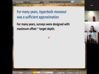
| 43:39 | many years, this was a sufficient . I would say for 50 |
|
| 43:45 | that was a sufficient approximation. And is it that what? Because surveys |
|
| 43:51 | designed where the maximum offset was about to the target depth. So if |
|
| 43:57 | looking for um a target about 10,000 down, you make a uh the |
|
| 44:04 | of uh of uh maximum offset is 10,000 ft. And so with |
|
| 44:13 | with that limitation, this limitation uh one of the, one of |
|
| 44:20 | assumptions that Dix made is approximately he assumed a small ray parameter. |
|
| 44:26 | if you limit the maximum offset, do limit the maximum ray parameter. |
|
| 44:33 | about the time I came into this , we invented a VL. And |
|
| 44:39 | we began to extend the surveys to offsets. Why is that? |
|
| 44:43 | if we want to uh uh use VO uh uh the longer uh |
|
| 44:50 | we have the more amplitude variation with , we're gonna have and so we |
|
| 44:56 | to have longer offsets. Well, thing we found is that our hyperbolic |
|
| 45:04 | was not sufficient. I remember I the one inside Amma who discovered |
|
| 45:13 | And my boss said, you I've, I've sort of been wondering |
|
| 45:17 | that and uh congratulations, you explained us why uh the hyperbolic equation do |
|
| 45:25 | work for long offset because uh uh violated the, one of the assumptions |
|
| 45:31 | we made. And so uh what need to do uh is uh find |
|
| 45:36 | better approximation than the hyperbolic move out . So let me just show you |
|
| 45:43 | picture of that here is actual data AOL. And uh and from those |
|
| 45:49 | days, by the way, th is probably um um 25 years |
|
| 45:54 | And so here we have a time and you can, and this is |
|
| 45:58 | data and you can see that the has been flattened uh at uh um |
|
| 46:04 | for short offsets. And uh uh further off, this is not |
|
| 46:13 | And furthermore, uh uh can you here at, at deeper uh uh |
|
| 46:19 | layers, it's flatt for further offsets this, this layer is flat for |
|
| 46:25 | offsets, but this one begins to right about here. And furthermore, |
|
| 46:30 | loses the uh frequency right here. what should we do about that? |
|
| 46:36 | , so there was a smart uh a friend of mine uh uh |
|
| 46:41 | too bad. He's now deceased. uh uh uh His name was |
|
| 46:46 | This was a student of his and said, well, you know, |
|
| 46:50 | looking back at the derivation that we for the uh hyperbolic equation, we |
|
| 46:56 | some uh tailor approximations there. So just add another term to the tailor |
|
| 47:03 | approximation. Remember uh uh uh go and check about the discussion in math |
|
| 47:10 | about the tailor approximation. And you'll that what we did before was equivalent |
|
| 47:15 | assuming uh that uh uh uh uh when you have a function um um |
|
| 47:25 | function of, of uh here's a function. But let's talk about a |
|
| 47:29 | function, the square of the time talk about that as a function of |
|
| 47:35 | that has a value at zero offset by this. And the variation with |
|
| 47:41 | that we derived from uh using Taylor's to come up with the hyperbolic |
|
| 47:47 | Our equation was we added this term and this is a little bit different |
|
| 47:52 | than we had before. But you see that's exactly what we had |
|
| 47:55 | And so what Taylor said was if not good enough for you, you |
|
| 48:01 | add another term which is the has see th this term is non |
|
| 48:06 | let's just take that same term and it and then add another parameter |
|
| 48:10 | And then you can do that again again, if you want. And |
|
| 48:14 | uh let's just add a term like . And so what is this quantity |
|
| 48:19 | to star that's here is a to uh in, in terms of quantities |
|
| 48:25 | we've already defined uh uh uh R velocity. But look at this, |
|
| 48:31 | is something called R MS four. is that here is RM four. |
|
| 48:37 | is a, a, an average of like the R MS average, |
|
| 48:41 | that it involves the average of the power of velocity. Whereas when we |
|
| 48:49 | with the uh R MS average, an average of the square velocity. |
|
| 48:58 | . So uh uh this quantity obviously be computed from these right. Uh |
|
| 49:04 | uh uh If you take this um uh uh literally as uh dix |
|
| 49:12 | you can uh uh decide what are these in these interval velocities in the |
|
| 49:18 | all the way down from the top the bottom. And then you can |
|
| 49:22 | uh calculate this quantity using those same . It's obviously gonna be a different |
|
| 49:29 | when you end up. Uh oh the way, this is the fourth |
|
| 49:32 | just like this is the second power RMX because you can see it, |
|
| 49:37 | has the dimensions of velocity squared. this one has dimensions of velocity of |
|
| 49:42 | . So this is the fourth And if we want to know what |
|
| 49:45 | RM four by itself, we just the fourth the of the inverse fourth |
|
| 49:51 | of this. No. Now, this seemed like a very good |
|
| 50:03 | Uh I just recognize that we might , I see here. Sorry, |
|
| 50:09 | should have, you should have interrupted . Uh uh uh There's my leisure |
|
| 50:18 | . OK. So, so you see this, uh uh this |
|
| 50:23 | RM four appears in the expression for to star, which is in |
|
| 50:27 | And you can see the weak and principle calculate this from quantities already known |
|
| 50:34 | we just go ahead and do the . But it's gonna be subject to |
|
| 50:40 | assumptions that we already made. And those assumptions were wrong, maybe this |
|
| 50:46 | the wrong thing to do. But uh this is what um uh Tanner |
|
| 50:52 | . So now, uh it seemed a good idea but um uh what |
|
| 50:57 | means is look at it carefully, is at, at, at large |
|
| 51:04 | . This means that the square of increases according to the fourth power of |
|
| 51:09 | which is not physically reasonable. Uh uh uh at large RS of |
|
| 51:15 | this term is gonna dominate uh this because this has X to the fourth |
|
| 51:20 | there. And so we're gonna have squared increasing to the fourth power off |
|
| 51:25 | . So that's not what we But so in 1995 a colleague and |
|
| 51:35 | owes this modification of the Tanner and uh uh algorithm, we said, |
|
| 51:42 | just uh use our physical intuition and without appealing to um to uh Taylor |
|
| 51:49 | all, we're just gonna add a in here, add a chart and |
|
| 51:55 | gonna be one plus a term which as the square of offset. And |
|
| 52:01 | gonna be choosing a so that we have so that we get the correct |
|
| 52:06 | long offsets. And uh uh we very proud of ourselves for this. |
|
| 52:11 | uh You, I'll show you what , uh we did uh at large |
|
| 52:16 | uh this uh uh becomes this. um uh why is that at large |
|
| 52:29 | , this term dominates the one. so uh uh X squared takes away |
|
| 52:35 | of these X's here. And so left with X squared again. So |
|
| 52:40 | , so I, so at large , we, we do get square |
|
| 52:46 | increasing with a square of offsets but a different velocity and it's not gonna |
|
| 52:51 | the R MS velocity, it's gonna a different velocity depending on the value |
|
| 52:56 | A. And so we're gonna define , in terms of the horizontal velocity |
|
| 53:02 | . If you put that in then at the largest uh uh |
|
| 53:08 | uh uh the square of time is according to the square of offsets with |
|
| 53:12 | horizontal velocity rather than the R MS . So, we were very proud |
|
| 53:18 | Marsa. So, um uh uh so we showed this to our colleagues |
|
| 53:34 | Amaco and they said, oh, , what is the horizontal velocity |
|
| 53:39 | we don't know the horizontal velocity. uh uh And so we said, |
|
| 53:45 | , uh let's think about that. , uh who want to derive the |
|
| 53:50 | velocity in the terms that we've already ? That is we already know uh |
|
| 53:55 | the assumptions that dick made, we all the layer thicknesses and all the |
|
| 54:00 | uh uh all the local velocities. so previously, we had found these |
|
| 54:07 | exact expressions, these are before, we made um uh any tail expansion |
|
| 54:15 | , you go back and uh uh , let's see here. Oh |
|
| 54:21 | Uh If, if we were doing with an SCG version of this |
|
| 54:26 | we would just click on this uh link here and it would take us |
|
| 54:30 | a few slides. You'll have to back yourself in the files and find |
|
| 54:36 | we started with these two exact And uh uh then at that |
|
| 54:43 | we found the limiting solutions here for and Great Proctor. Now we're gonna |
|
| 54:48 | uh seek the limiting solutions at right Proctor. So we're gonna define |
|
| 54:55 | uh uh the horizontal velocity as the of offset divided by time in the |
|
| 55:02 | where the angle approaches 90 degrees. putting in uh all these uh uh |
|
| 55:10 | the uh for uh the offset and the arrival time, the expressions that |
|
| 55:16 | found before. Uh we can uh see what we do. Oh |
|
| 55:23 | we uh we substituted for the ray that this is the definition of the |
|
| 55:34 | part stuck that right in there. uh then we used Lopes rule, |
|
| 55:42 | know. So first let me uh you the name of the Lopes |
|
| 55:49 | That's a French name. And it looks if you were, if |
|
| 55:53 | were an English name, you would hospital. But in French that's pronounced |
|
| 55:59 | and the man's name is loyal with an L and um oh quotation mark |
|
| 56:10 | . So, uh let me ask uh the class uh Lily, do |
|
| 56:15 | , do you know lo pal's OK. Uh So uh uh a |
|
| 56:22 | already uh uh I'm uh given the that some of the class doesn't know |
|
| 56:32 | loyal. So I think I, we're a bit behind schedule right |
|
| 56:38 | I, I don't want to um back to math 101. But if |
|
| 56:43 | , after class you go back to 101 and you'll or maybe to the |
|
| 56:49 | . Yeah, go to the glossary you will find under the L's parts |
|
| 56:53 | , of the glossary, you'll find and loyal is uh uh uh uh |
|
| 57:04 | uh local rule is AAA way for to deal with a situation where you |
|
| 57:11 | zero divided by zero. So uh here in, in this formula at |
|
| 57:18 | near to uh uh 90 degrees cosine is near to zero. So we |
|
| 57:27 | uh uh we have zero here. in the numerator and the denominator. |
|
| 57:33 | uh so we have infinity here, we have another infinity here. So |
|
| 57:39 | is infinity divided by infinity? so uh that's the problem that was |
|
| 57:44 | by loyal in the 19th century. you will see the answer given there |
|
| 57:50 | the glossary and using loyal though, able to, to convert this thing |
|
| 57:57 | this. And you can see here this is the average value of the |
|
| 58:03 | uh uh uh uh this is the value uh uh of the local |
|
| 58:10 | It, it differs from the R uh uh average. So this is |
|
| 58:15 | a of meric average and that is horizontal velocity. So I'm gonna leave |
|
| 58:20 | to you all to uh go back , and uh and, and uh |
|
| 58:25 | go back to uh the glossary and loyals rule and you'll then convert this |
|
| 58:33 | , which is pretty messy, I say to this expression, which is |
|
| 58:37 | simple. And then you'll recognize that is simply the arithmetic average velocity. |
|
| 58:49 | now uh the uh the ab we'll this the abnormal move out equation. |
|
| 58:55 | uh uh uh when we had the move out equation, that's often called |
|
| 58:59 | normal move out equation. So we're call this the abnormal move equation. |
|
| 59:05 | means not normal. And so uh it is and everything is specified. |
|
| 59:12 | uh so, oh you can uh uh you can calculate everything in here |
|
| 59:23 | uh by observing how the R MS changes with depth. So, |
|
| 59:31 | it is common to regard a to as empirically determined, just like we |
|
| 59:37 | the NMO velocity. See right back , we had the R MS velocity |
|
| 59:42 | , and now we have the no here and we're gonna empirically determine another |
|
| 59:47 | a of star. And I can you it's gonna be different. Now |
|
| 60:02 | these corrections, the move out can flattened out to longer offsets. And |
|
| 60:07 | practice, it is frequently asserted that calculate coefficient A on previous rate is |
|
| 60:13 | sufficient to flatten, gather it very out ie not as far out as |
|
| 60:18 | a ratio of two. When you to maximum offsets as far as two |
|
| 60:24 | the target depth, you um uh previous expression does not work. And |
|
| 60:31 | what we're gonna need in uh in case is anti oxen. So that's |
|
| 60:37 | than 10. So let's have a . Uh li li is this statement |
|
| 60:47 | or false? You think it's Let's read it carefully for a single |
|
| 60:54 | D isotropic layer but not. Uh , you know, I if you |
|
| 61:05 | back and, and uh look at um uh at the discussion and you'll |
|
| 61:10 | that in that case where it's a single one B isotopic layer, |
|
| 61:15 | It's simply the uh the hyperbolic moveon is simply a statement of the Pythagorean |
|
| 61:22 | from plane geometry. So that would true. Um So uh Carlos it |
|
| 61:36 | the Hyperbolic move out equation is an based on the assumption that the rays |
|
| 61:42 | straight. Is this true or I think that is true. Professor |
|
| 61:48 | . Uh uh This is a AAA question. It can be thought of |
|
| 61:52 | way except that that's not how we it. We did not derive it |
|
| 61:58 | that the rays are straight because we the rays are not straight. Uh |
|
| 62:02 | We assume that uh using the assumptions uh you know, one day isotropic |
|
| 62:08 | and small ray parameter. And so is that um statement of assumptions was |
|
| 62:15 | explicitly about five or 10 slides So this statement is wrong. |
|
| 62:23 | Mhm uh So versa. Is this ? I think this is not |
|
| 62:37 | Uh uh So uh I think that Carlos answering. So, what did |
|
| 62:41 | say Carlos? Yeah, they say not, it's not connected right |
|
| 62:45 | I don't know why but I yeah, we were, we were |
|
| 62:48 | that this is false most of the . Yeah. Th this is |
|
| 62:53 | Uh uh But many times uh you might find uh some cases where |
|
| 62:58 | true, but usually you're gonna find it's false. OK. So uh |
|
| 63:07 | Rosa uh can you hear me? that? Yes, Rosa. Can |
|
| 63:13 | hear me? Yeah. Uh are you um she, she's not |
|
| 63:20 | ? She's not online. Oh She's online. Ok. So I had |
|
| 63:25 | . Uh OK. So uh we'll turn to um uh Lily. |
|
| 63:29 | So uh uh what it says here the abnormal neuro equation uh in, |
|
| 63:35 | quotes. Oops, let me get um pointer. I don't know how |
|
| 63:40 | lose this pointer. Give me a . Yeah. Yeah, we say |
|
| 63:51 | back online right now. Oh welcome back. Uh uh Thank |
|
| 63:57 | Sorry. Something with my connection. . Uh So you're just in |
|
| 64:01 | So this question is for you. uh It says uh the abnormal move |
|
| 64:07 | equation, true or false is just second order tailor expansion in X |
|
| 64:13 | So it could be called the fourth move out equation. Is this true |
|
| 64:17 | false? Uh I am not sure true. Well, remember what we |
|
| 64:31 | about. I remember I showed the of uh uh a tanner with a |
|
| 64:35 | in his mouth. Uh So, so that um uh that slide showed |
|
| 64:43 | uh 1/4 order uh move out That was what he posed, but |
|
| 64:48 | not very good, it's not physically . And, and instead of better |
|
| 64:53 | uh uh uh a better um uh uh was given by uh Twin and |
|
| 65:01 | . And that's what we call the liard equation. And it differs from |
|
| 65:06 | second order Taylor expansion uh by having , a physically motivated correction term in |
|
| 65:13 | denominator of the final term. And that was what corrected the uh the |
|
| 65:21 | the travel times that far off sets to have the correct functional form. |
|
| 65:27 | because of that, because of that physically motivated correction factor, uh that |
|
| 65:37 | is not just a second order tailor . So the answer to this one |
|
| 65:42 | not as false. OK. Uh to you Lily. So uh it |
|
| 65:55 | has a better approximation. The abnormal out equation has from each vertical travel |
|
| 66:01 | T zero. It has um uh empirical parameter, 23 or a three |
|
| 66:09 | quantities calculated from these. Uh So le let's go these uh one at |
|
| 66:16 | time. Um uh As a matter fact, what I'm gonna do is |
|
| 66:20 | gonna uh put Lee Lee on the for uh uh for A and I'm |
|
| 66:26 | go to Carlos for, on the for B and I'm gonna go to |
|
| 66:31 | on the spot for C. Lili uh does it have one empirical |
|
| 66:37 | plus quantities calculators from this? So think it's three? OK. So |
|
| 66:45 | , so you, you jump to right uh uh to the right answer |
|
| 66:49 | uh right away. So uh guess Carlos you're off the hook, guess |
|
| 66:55 | ? You're off the hook, you Lili a cup of coffee. Uh |
|
| 66:58 | time you see her because she answered your behalf. OK. Well done |
|
| 67:05 | . So now, um so you that what we've been looking at is |
|
| 67:13 | the simplest of all possible problems. so now we wanna look at uh |
|
| 67:18 | some complications that can arise. And let's look at interfering ways. |
|
| 67:25 | so as we learned before, when have the sum of two solutions, |
|
| 67:29 | also a solution. So for for the scalar wave equation, if |
|
| 67:35 | have this for uh one solution would one. And if P two is |
|
| 67:40 | a solution, then the sun is a solution. And what this means |
|
| 67:45 | that um uh you can, that you can have many solutions uh a |
|
| 67:53 | synthesis thou thousands of times like that the, as um described by Mr |
|
| 68:01 | . And they have gonna have different and frequencies that is still a |
|
| 68:08 | Now, since any solution of the equation can be separated into those |
|
| 68:14 | these can be a uh uh a separately. And what that means is |
|
| 68:20 | intersecting waves which have different sources, wave vectors, et cetera, et |
|
| 68:25 | simply superpose then pass on without So I have a, a cartoon |
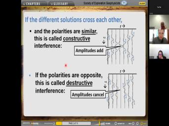
|
| 68:33 | . So uh uh look at this uh with uh uh uh uh |
|
| 68:39 | this wave going down and this way coming up at the first time here |
|
| 68:47 | the, at the, at the time this wave has gone down, |
|
| 68:51 | wave has gone up at the next uh that continues and you see at |
|
| 68:57 | point they begin to overlap, begin overlap. And at this time, |
|
| 69:04 | peak, the ongoing peak exactly is at the same time as this upcoming |
|
| 69:09 | . And guess what? It made single peak with twice the amplitude. |
|
| 69:15 | then this wave here which is going , continues up and this wave here |
|
| 69:21 | was going down, continues down They are. And you see at |
|
| 69:26 | more time steps they have separated. , so uh this is what happens |
|
| 69:33 | when the two waves are passing each , when the polarities are the same |
|
| 69:39 | similar, see right there, the amplitudes add together. And by the |
|
| 69:49 | , you see that, that uh trough is uh uh uh uh uh |
|
| 69:54 | is a trailing trough and this is leading trough. This difference in time |
|
| 69:59 | the same as this difference in time . So these two waves simply add |
|
| 70:05 | making this single um uh this single with twice the amplitude. Now what |
|
| 70:15 | if the amplitudes are opposite? So one going down is the same, |
|
| 70:21 | , this one going up as a um clarity, you see the peak |
|
| 70:28 | a negative peak, whereas up here the peak was a positive peak. |
|
| 70:32 | the same thing happens, they get and closer and guess what at at |
|
| 70:38 | they are exactly on top of each , they exactly cancel out. So |
|
| 70:44 | looks like nothing is happening. But course, inside here, uh the |
|
| 70:49 | atoms are still moving the uh the and so after the um uh uh |
|
| 70:58 | at the next time step, this false going up is still going |
|
| 71:04 | you see it emerges on the other without uh uh being changed. And |
|
| 71:09 | positive one going down that emerges on other side and they separate just like |
|
| 71:15 | were before. Except that now the pulse is down here and started off |
|
| 71:21 | here. So here the amplitudes So this happens because of the linear |
|
| 71:32 | of the wave equation. And it's of puzzling. I mean, when |
|
| 71:36 | look at this seismic gram right you say, well, there's no |
|
| 71:40 | present, but in fact, there's ways present which exactly cancel each other |
|
| 71:45 | at this point in time. But have momentum and they have the, |
|
| 71:49 | atoms are still moving and uh uh uh they come out the other side |
|
| 71:55 | that. Now, uh here's a , we have been assuming that uh |
|
| 72:05 | uh as we derive the wave we use Taylor's approximation several times. |
|
| 72:11 | in there, we assume small amplitude displacement. And so if the displacement |
|
| 72:18 | is uh as large, then uh I just told you is not |
|
| 72:25 | then there can be nonlinear effects which not included here since we uh uh |
|
| 72:31 | at the beginning that the strains are . So you can go back at |
|
| 72:35 | beginning of our uh derivation of the equation, the, the, |
|
| 72:40 | the waves are small, that's how got to have a linear equation. |
|
| 72:47 | uh all sorts of good things come of uh uh of uh linear |
|
| 72:54 | And that's one of them. yeah, uh uh if it's not |
|
| 73:02 | , if the amplitudes are large, there's all kinds of uh of, |
|
| 73:07 | other stuff can happen. But we're gonna discuss this uh in this course |
|
| 73:13 | uh our time is limited. So Carlos, this one comes to |
|
| 73:19 | Yes, when waves collide, they with one another, just like billiard |
|
| 73:24 | on a table and they conserve energy momentum in the collision. Is this |
|
| 73:30 | or false? They think it's true . No, no. Look at |
|
| 73:36 | . Look at this right here. had these two waves collide and they |
|
| 73:41 | , they didn't bounce off of each this way going down here and this |
|
| 73:46 | is going up here. They, did not bounce off of each |
|
| 73:51 | Um Is that so uh waves are like particles, they're not like builder |
|
| 73:59 | . And I can tell you that at the beginning of the last |
|
| 74:03 | there was a lot of discussion in physics community are are light waves waves |
|
| 74:09 | are they particles? And uh uh it was a tremendous um revolution in |
|
| 74:21 | in physics because at that time, had good proof that uh waves were |
|
| 74:28 | light cause waves and everybody was pleased themselves, you know, that, |
|
| 74:35 | was uh established by uh uh Maxwell's for electromagnetic waves. Everybody was pleased |
|
| 74:42 | them be themselves because they um uh them, but they had proved that |
|
| 74:52 | was made out of waves. By way, Isaac Newton didn't believe that |
|
| 74:56 | Newton thought that that uh uh light particles. You know, he was |
|
| 75:02 | brilliant guy, one of the, greatest uh scientists of all time and |
|
| 75:07 | was wrong on this point and Maxwell him uh uh wrong. And so |
|
| 75:14 | was very pleased with themselves except that showed in 1905 that sometimes light acts |
|
| 75:23 | particles. And by the 19 uh uh uh the theory was fully |
|
| 75:29 | of quantum mechanics where we understand that quantum mechanics, light sometimes acts like |
|
| 75:36 | waves and sometimes like particles on the scale on the scale of atoms. |
|
| 75:45 | , in our business, we're not with that tiny scale so that we |
|
| 75:49 | in our business, we have uh sound waves acting like waves, not |
|
| 75:55 | billiard balls. OK? But they , they are still conserving the |
|
| 76:03 | Yeah, they are conserving. that, that's, that's uh that |
|
| 76:09 | that, that, that is true and energy. So this comes to |
|
| 76:15 | Brier when waves collide they superpose back , we said they interfere but uh |
|
| 76:22 | they superpose with amplitudes adding together then through each other like ghosts is |
|
| 76:28 | True. False, true. yeah, that's true. Now, |
|
| 76:33 | uh uh somebody might say, they, they, they don't always |
|
| 76:37 | it together. Let's go back to cartoon. So here's a, here's |
|
| 76:41 | example where they subtracted from each But uh subtraction is just like addition |
|
| 76:46 | a minus sign there. So I'm , uh uh I'm gonna say that |
|
| 76:51 | straight. OK. This one comes you uh uh relate when waves |
|
| 77:03 | they superpose with phases added together, pass through each other like ghosts, |
|
| 77:11 | or false. Now see you, not reading the question carefully. Let's |
|
| 77:16 | back to the previous question. So , your question really was the same |
|
| 77:20 | this question number two. But here amplitudes, here it says phases. |
|
| 77:27 | . So, so this one is whereas this one is true. Go |
|
| 77:31 | over what we, how we described . The phases don't add, it's |
|
| 77:36 | amplitudes of that. OK. So know that all of you have been |
|
| 77:42 | uh in your minds as we've been about PW. But let's consider now |
|
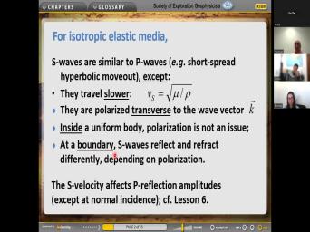
| 77:47 | wa OK. So isotropic elastic uh shear waves are similar to P |
|
| 77:59 | for example, they have short spread and Google except they travel slower. |
|
| 78:05 | The shear wave velocity is given by expression um uh Instead of the P |
|
| 78:10 | velocity expression, remember P wave velocity we had right here an M instead |
|
| 78:18 | a mu and we know from previous that M is equal to a plus |
|
| 78:25 | thirds mu. So that's obviously a n bigger number than mu. So |
|
| 78:29 | waves travel faster. Here's another um case of um similarity, the shear |
|
| 78:37 | are polarized transversely to the wave So, so this wave vector points |
|
| 78:43 | the direction the wave is traveling for waves uh uh the polarization that is |
|
| 78:49 | displacement is pointed in the same But in for sheer waves, it's |
|
| 78:54 | perpendicular plan. Now inside a uniform , uniform isotropic body, it's the |
|
| 79:06 | for all polarization. But at a , sheer waves reflect and refract differently |
|
| 79:13 | on the polarization. So that's uh uh you've heard the phrases sh waves |
|
| 79:23 | SV waves. So uh uh there uh the, the, the H |
|
| 79:29 | the V referred to the polarization vector to uh uh the horizontal direction or |
|
| 79:36 | vertical direction. And so, uh the body uh uh without any um |
|
| 79:45 | , without any reflecting boundary nearby both these waves travel at the same |
|
| 79:55 | even though gravity is there, Gravity is always pointed out. But |
|
| 79:59 | these waves are traveling with velocities which depend on gravity, they depend on |
|
| 80:06 | . And so uh inside a uniform body, those two waves vs and |
|
| 80:12 | uh VSH and VSV travel with the velocity. But when they hit the |
|
| 80:18 | , then they interact with the boundary as it says here, And |
|
| 80:24 | we can say that the sheer velocity of a medium affects the P wave |
|
| 80:32 | amplitude at, except at normal that's kind of amazing, isn't |
|
| 80:38 | Here? You have a P wave in to a reflecting boundary being reflected |
|
| 80:43 | a P wave. And yet even the properties of the sheer waves of |
|
| 80:48 | boundary helped to determine the amplitudes. that amazing? And so we're gonna |
|
| 80:55 | more about that in lesson six. that is the secret behind a |
|
| 81:04 | Now, usually we try to exclude shear waves from our P wave |
|
| 81:10 | I'm sure that uh uh you're familiar these ideas. So in, in |
|
| 81:16 | , uh there are no share waves uh uh share waves can't travel through |
|
| 81:20 | ocean. And so we're uh we're our data on hydrophone data in the |
|
| 81:25 | and there are no share waves. so uh that's a clever thing to |
|
| 81:29 | uh in the marine environment in land . Uh uh We usually put out |
|
| 81:35 | geophones only. Why is that? , lots of reasons. But one |
|
| 81:40 | is that the sheer body waves are recorded on vertical uh geophones that is |
|
| 81:48 | say whatever sheer waves are coming up the subsurface nearly vertically, they're tra |
|
| 81:55 | polarized transversely to that upcoming he And so that means the polarization is |
|
| 82:04 | horizontal so that it's not gonna record much on this Radical gear film. |
|
| 82:11 | uh it'll report some but not uh not a lot. And furthermore, |
|
| 82:17 | sources are designed to maximize P wave and to minimize two wave power. |
|
| 82:25 | an example of that. Normally these on land, we do not use |
|
| 82:30 | . When I first came into this , we did use dynamite and there's |
|
| 82:35 | lot of, lots of reasons uh we don't use dynamite anymore. But |
|
| 82:40 | reason is that it's dangerous. So learned a long time ago that uh |
|
| 82:46 | clever thing to do is use for , for sources on land. Uh |
|
| 82:53 | Oh Wow. Uh We're gonna use vibrator as it says here. But |
|
| 83:03 | the, the, you know, the cartoon says it's a horizontal. |
|
| 83:09 | let's look here at the vertical So we're uh we're making P waves |
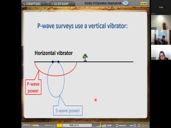
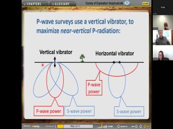
|
| 83:14 | vertical vibrators and that has maximum power the P wave is downwards. |
|
| 83:21 | we shouldn't call this a P wave because it does make shear waves. |
|
| 83:25 | maximum power for the sheer waves is and vertically. The sheer waves do |
|
| 83:32 | some power near vertical. They make power. Um um But so |
|
| 83:39 | that's why we shouldn't call this a wave vibrator. We should call it |
|
| 83:42 | vertical vibrator. And uh uh when , and that was, this was |
|
| 83:54 | a long time ago, uh when came for just about the same time |
|
| 83:59 | I came into the business in the 19 eighties. Uh uh we invented |
|
| 84:04 | vibrators uh to make uh um uh shear shear waves. And so the |
|
| 84:11 | vibrators maximize the power of the shear . Um oh uh uh down going |
|
| 84:21 | wave is in the vertical direction. shear wave is maximum and the P |
|
| 84:27 | power is maximum horizontal. You can that if you're vibrating horizontal here, |
|
| 84:32 | gonna be pushing a P wave out way and out this one. |
|
| 84:43 | Um No, why would we want have a horizontal library? Um The |
|
| 84:58 | we wanna have a horizontal vibrator is maybe we maybe uh you know, |
|
| 85:04 | had all these good reasons for minimizing wave in our data and those are |
|
| 85:12 | good reads. And sure enough, use those most of the time, |
|
| 85:17 | there might be other case, other where we actually might want to maximize |
|
| 85:23 | share waves. And so that's why invented horizontal library. And that was |
|
| 85:28 | by a company. Uh uh It , it was done by uh Conco |
|
| 85:34 | called Conocophillips. About the time that I came into this business now that |
|
| 85:44 | use more techniques for excluding she uh energy of uh from our P wave |
|
| 85:52 | . For example, in processing, gonna get sheer waves on our vertical |
|
| 86:01 | fault created by our, our uh vibrators. Anyway. And most of |
|
| 86:09 | uh shear waves arrivals are surface waves called ground wall. And it's traveling |
|
| 86:15 | horizontally parallel to the surface and vibrating . So those um uh uh those |
|
| 86:26 | are gonna be strongly uh recorded on uh instruments. And so we wanna |
|
| 86:33 | rid of those. And so uh do we do those? Uh we |
|
| 86:38 | uh use a technique called FK filtering I think we're gonna talk about, |
|
| 86:42 | think the professor Joe is gonna talk you about FK filtering. And then |
|
| 86:47 | way is to uh uh to stack we filter these out, we're gonna |
|
| 86:54 | and migrate with P wave velocities. so that means we're gonna make |
|
| 86:59 | the P wave arrivals reinforce each other the sheer wave arrivals cancel each other |
|
| 87:05 | by these techniques. OK. um before we leave this topic of |
|
| 87:17 | waves, I wanna say for anisotropic , there are many new shear wave |
|
| 87:29 | . No, it says all rocks are an I should drop. And |
|
| 87:33 | most of our data is P wave , there is no point in discussing |
|
| 87:38 | shear waves further, we're gonna talk an isotropic shear waves in less than |
|
| 87:49 | . OK. So that's all we're say about sheer waves at this |
|
| 87:55 | So uh coming to you uh Carlos is this true or false sheer waves |
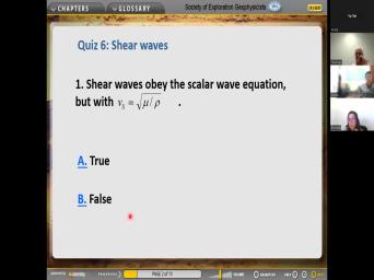
|
| 88:03 | the scalar wave equation with this sheer velocity. Is that true or |
|
| 88:09 | That is true for us? now think about that um uh of |
|
| 88:19 | scalar wave equation uh was in a equation and the scalar phi and it |
|
| 88:26 | say anything about polarization. Mhm So would say this is false because it |
|
| 88:36 | the vector wave equation with this Yeah. So if you go back |
|
| 88:43 | look at at um oh uh what , how we derive uh the vector |
|
| 88:49 | equation for shear waves, you'll see a, it's an equation with |
|
| 88:53 | not the scale. So uh So uh this is a good time |
|
| 88:59 | me to remind you all that when doing the final exam, you have |
|
| 89:04 | have plenty of time. So you look at this uh uh If you |
|
| 89:08 | this question, a question like this the final exam, you should |
|
| 89:11 | oh I think I know the But let me go, let me |
|
| 89:15 | back and see what, how we the v the, the wave equation |
|
| 89:20 | sheer velocities for sheer waves. And see that it's a vector wave |
|
| 89:25 | So you immediately know this one is . OK. So, uh for |
|
| 89:32 | bead, is this true or You have a P vibrator. Uh |
|
| 89:38 | it does not generate share ways, or false, it's false. |
|
| 89:42 | it's false. Uh uh We talked that explicitly. Uh uh it generates |
|
| 89:47 | P waves, also share ways. uh um uh so uh because it's |
|
| 89:53 | vertical mark, that's a better way describe it. OK. I shall |
|
| 90:02 | , says inside an isotropic formation. waves propagate just like sh waves except |
|
| 90:10 | the difference in polarization. Is this or false? You say false? |
|
| 90:17 | what are uh uh tell me what's about this? What that uh |
|
| 90:30 | So uh it says except for the . So except for that polarization |
|
| 90:37 | what we said before is they have same velocity. Yeah. So this |
|
| 90:42 | be true. OK. So we've done P waves and we've done |
|
| 90:51 | waves. Now, we're gonna combine to do converter waves. So we're |
|
| 90:57 | learn in lesson six that when we uh a reflecting horizon, we're gonna |
|
| 91:04 | converted waves. Here's an incoming P and we have a reflected P wave |
|
| 91:10 | a reflected shear wave and a transmitted uh P wave and a transmitted shear |
|
| 91:17 | . So these sheer waves coming out a reflecting horizon uh uh happen uh |
|
| 91:29 | at uh a boundary between um elastic . If it's uh of course, |
|
| 91:36 | it's a boundary between two fluids, there's no share waves at all. |
|
| 91:40 | if there's ela elastic, if there's mediator or, or rocks, we're |
|
| 91:45 | get conversions here. And it's a thing if we have an incoming SG |
|
| 91:51 | . But this is uh the, , the normal situation here, incoming |
|
| 91:56 | wave, outgoing four waves here. we've gotta have conversion of a conservation |
|
| 92:05 | energy going, we can't have any being left behind. So that means |
|
| 92:12 | uh that uh uh we, we to, we have to get, |
|
| 92:19 | have to get the energy for these she waves from that reflected P wave |
|
| 92:25 | the reflected transmitted P wave. So why the P wave A O has |
|
| 92:32 | shear modulus in the reflectivity. where do we use these converter |
|
| 92:42 | Uh uh They're uh important in two . One is ocean bottom seismic and |
|
| 92:48 | is sheer wave logging. OK. , um first let's talk about ocean |
|
| 92:55 | seism. So here's a cartoon of of an ocean bottom seismometer sitting on |
|
| 93:01 | sea floor. And we're gonna have conventional source up here at the |
|
| 93:06 | And we're gonna be uh we wanna an image of this reflector down |
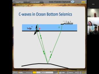
|
| 93:12 | So only gonna be able to make waves coming out of this source. |
|
| 93:18 | here's the P wave coming down reflecting back up to the receiver. And |
|
| 93:24 | can see the receiver has three vector and one hydrophone component. So it's |
|
| 93:30 | a four component receiver. So there's more thing that happens here. Some |
|
| 93:36 | the energy that comes with this reflection past the sea floor up to the |
|
| 93:42 | surface reflects back down and hits the again with a, a two day |
|
| 93:49 | , a two way delay coming from month. So that's why we have |
|
| 93:57 | uh uh the hydrophone in here. by uh by being clever, we |
|
| 94:04 | combine the data from uh the hydrophil from this vertical com uh vertical component |
|
| 94:11 | the GEO O to eliminate this water multiple. So we don't get interference |
|
| 94:19 | the multiple and the primer. So uh that's a topic outside of the |
|
| 94:26 | this course. But you can see in principle, we do wanna get |
|
| 94:31 | of one or the other and normally want to get rid of the water |
|
| 94:36 | multiple of the water, the surface and leave only the primary. The |
|
| 94:43 | we do that is by a certain uh combination of the hydrophone and the |
|
| 94:49 | geophones. But there's something else that here. Some of this energy is |
|
| 94:56 | be converted to shear wave energy come here and it's gonna come back |
|
| 95:02 | Um uh uh uh polar is transversely this upcoming shear wave. So it's |
|
| 95:09 | register on mostly on the two horizontal and then they, they might not |
|
| 95:17 | aligned um uh in the, in uh plan of the figure like |
|
| 95:22 | But uh you can see that they're both be, that's why we need |
|
| 95:26 | of them so that we can uh all the upcoming shear wave energy. |
|
| 95:32 | , there is another conversion mode which here when the uh uh uh the |
|
| 95:41 | happens at the reflecting horizon, not the sea floor. And it turns |
|
| 95:48 | that this one usually is much more than this one for reasons involving rock |
|
| 95:55 | , this conversion is usually we and one is strong. And so we |
|
| 96:02 | conventionally call this one converted at the , we call that the sea |
|
| 96:11 | So uh this has been known uh for a long time. And so |
|
| 96:16 | AAA cartoon picture of that situation isotropic layer, uh flat reflector down here |
|
| 96:25 | show here, a B wave reflecting the midpoint and a sea wave reflecting |
|
| 96:32 | here at what's called the conversion So this previous reflecting point is reflecting |
|
| 96:42 | the midpoint. That's a geometrical That's just geometry. It's, it's |
|
| 96:48 | one half. But over here, conversion point is determined by Snell's |
|
| 96:55 | And Snell's Law works to make sure here's Snell's Law uh uh uh shown |
|
| 97:01 | this way, the sign of this angle divined by the sign of the |
|
| 97:07 | angle is equal to the ratio of velocities. So this conversion point |
|
| 97:17 | the uh the, the conversion which gonna be received here at X. |
|
| 97:22 | gonna happen at X of C following Law. And you see this is |
|
| 97:27 | physical argument, not a geometrical Uh So it's gonna make things |
|
| 97:39 | It means that in order to even where this thing is uh oh |
|
| 97:47 | we have to know the velocities or least we have to know the velocity |
|
| 97:52 | . Whereas to do a P wave for the P wave, we, |
|
| 97:56 | don't, uh we're gonna say this converts at uh this reflects at the |
|
| 98:03 | . And we don't need need to the velocity the P wave velocity to |
|
| 98:07 | that we can just say, of , it's gonna be reflecting at the |
|
| 98:12 | . So this is a more complicated . OK. So when you work |
|
| 98:19 | the implications of this, what you is that the image point offset varies |
|
| 98:26 | the depth of the reflector. So a uh a simple situation where the |
|
| 98:31 | velocity and the sheer velocity everything is with depth. And uh um here |
|
| 98:38 | have uh a source and receiver and midpoint is here, all the P |
|
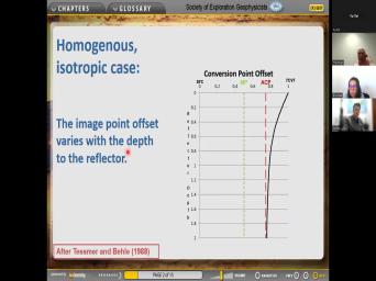
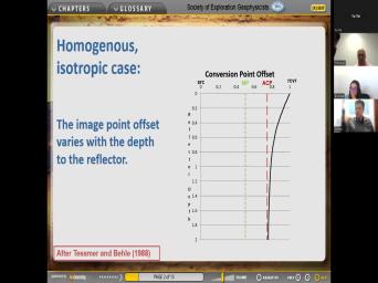
| 98:42 | are gonna be uh uh P waves off of any one of these layers |
|
| 98:47 | gonna be reflecting here at the But for this event here, which |
|
| 98:52 | converting at this layer here, um that's gonna be converted uh here and |
|
| 99:02 | up to the receiver. And if trace out all of the uh um |
|
| 99:06 | conversion points all the way down, gonna follow this black curve here. |
|
| 99:12 | so you can see that at large , it converges asymptotically to this point |
|
| 99:20 | , which we call the asymptotic conversion , asymptotic conversion point. And so |
|
| 99:27 | is uh uh done uh non So this means either great depths or |
|
| 99:34 | shallow times, either a great depth Charlton. Uh So, because of |
|
| 99:45 | variation of the, so the, , the conversion point is gonna be |
|
| 99:50 | at for every one of these layers here. And so you can't sort |
|
| 99:57 | traces into a common uh uh uh can't do what you do with P |
|
| 100:10 | for P waves. If you want have a, a AAA common reflection |
|
| 100:15 | gather, it's the same as a midpoint gather. But for converter |
|
| 100:19 | you can't do that with a simple operations. You have to know both |
|
| 100:25 | throughout the overburden. And in order calculate a common conversion point gap, |
|
| 100:35 | normally to do these to determine these , you need to have a common |
|
| 100:41 | part gather. So you need to this gather to get the velocities and |
|
| 100:46 | have to have the velocities to get . So you have to do an |
|
| 100:50 | workflow. It's complicated. So, uh I'm, I'm thinking that uh |
|
| 100:58 | know, at this point, none you students. And I'm thinking you |
|
| 101:03 | also uh uh you never worked with wave data. Is that correct? |
|
| 101:09 | . So uh uh you can see here that it's uh a lot more |
|
| 101:14 | than P wave data. And so have to have a good reason to |
|
| 101:18 | it. You wouldn't uh you uh you, you wouldn't do |
|
| 101:22 | In most cases, in most you want to, you know, |
|
| 101:26 | the converted waves in the same way we suppress sheer waves. Uh So |
|
| 101:31 | wanna concentrate on P waves. But , in other, in uh some |
|
| 101:36 | , you actually want to look at converter waves uh especially and uh we'll |
|
| 101:42 | some uh cases like that during this . Yeah. No, I want |
|
| 101:54 | return to this and I want to uh to talk about this asymptotic conversion |
|
| 102:06 | . There's a simple formula. So define some notation, let's have the |
|
| 102:12 | of the vertical velocities and we'll have ratio of move out velocity, call |
|
| 102:18 | gamma zero, call this gamma move ratio of vertical lo and then this |
|
| 102:23 | effective is defined to be the square the move out ratio divided by the |
|
| 102:30 | ratio. Then the asymptotic conversion point given by gamma effective, divided by |
|
| 102:41 | plus gamma effective. It's a simple uh with but uh to know that |
|
| 102:47 | have to know all these other things you don't know these when you first |
|
| 102:52 | begin to process the data. So have to do an iterative process for |
|
| 102:59 | learning how to uh uh uh uh all these things and then compute where |
|
| 103:06 | conversion points are happening, right? uh Just think about this, you |
|
| 103:12 | a source and you have a receiver you receive a converted wa where did |
|
| 103:17 | , where did it convert? You're imaging that part of a |
|
| 103:21 | where did it convert? Or you know if it's a P wave |
|
| 103:26 | you know, because it's at the but uh for a converter wave survey |
|
| 103:30 | don't know. So you got to this elaborate um uh computation to even |
|
| 103:37 | out what you're looking at. So about the move out velocity? So |
|
| 103:48 | for short offsets, the move out hyperbolic, just like we had for |
|
| 103:53 | waves, except that it's got the C wave move out velocity in |
|
| 103:59 | . And now that C wave move velocity is can be can uh it |
|
| 104:04 | be constructed from the P wave move velocity and the she wave move out |
|
| 104:09 | with these gamma functions. And remember gamma subzero is the ratio of the |
|
| 104:16 | of the VP to vs for vertical zero A. And the reason I'm |
|
| 104:25 | you this complicated formula is that you encounter even today, you might encounter |
|
| 104:33 | uh uh papers or references to a formula which in the different formula, |
|
| 104:41 | square of the C wave move out is equal to this product of P |
|
| 104:46 | PNML and SNML. Um uh but only true for a uniform isotropic layer |
|
| 104:54 | that's not true in uh in OK. Next topic is uh is |
|
| 105:06 | . So the the amplitude of the waves are zero for normal instance. |
|
| 105:12 | just think of a P wave going and converting to sheer waves coming back |
|
| 105:17 | . But if it's, if the wave is traveling vertically, it doesn't |
|
| 105:23 | whether the upcoming shear waves should be this way or polarized that way. |
|
| 105:28 | it doesn't do either one. It back with zero amplitude for the converted |
|
| 105:33 | at normal incident. It has opposite for positive and negative offsets. |
|
| 105:41 | if you have your uh uh uh uh can, can you see |
|
| 105:46 | my hand here, I've got my hand shy as a ocean bottom |
|
| 105:51 | receiver sitting on the sea floor and got my source over here coming down |
|
| 105:55 | a P wave and it's gonna, be hitting this uh uh um |
|
| 106:02 | it's go, it's gonna come down then come back up and it's gonna |
|
| 106:07 | a AAA, it's gonna have Oh it's, it's gonna be hitting |
|
| 106:18 | receiver like this at an angle. so it's gonna be picking the receiver |
|
| 106:24 | my right. Meanwhile, if uh then uh uh I shouldn't say |
|
| 106:31 | suppose the, the source boat keeps coming on over here, coming on |
|
| 106:36 | here and eventually it gets to where source boat is over here. |
|
| 106:40 | the key wave goes down, reflection back up and kicks the uh the |
|
| 106:46 | the other way. So that's what mean when I say here, it |
|
| 106:50 | opposite polarity for positive and negative right? This polarity reversal is a |
|
| 107:01 | of the scale of reciprocity there, we talked about before, which says |
|
| 107:07 | scale of reciprocity theorem says that interchange and receiver that leaves the data |
|
| 107:13 | So obviously, uh uh in, a case, like I just showed |
|
| 107:16 | here for opposite polarity, uh uh not true. The two side, |
|
| 107:22 | you have a common midpoint gather of a common conversion point gather, that's |
|
| 107:28 | to make. But a common midpoint is easy to make. And |
|
| 107:36 | uh when you, uh so, you're expecting that far up. |
|
| 107:42 | the two halves of that common midpoint to have opposite polarity on your workstation |
|
| 107:52 | . So it's common in split spread to multiply one side by minus |
|
| 107:56 | So they can easily stack it and it. OK. That's been understood |
|
| 108:03 | a long, long time. This of uh um a clarity difference on |
|
| 108:09 | two sides of uh of the of midpoint gather. But let me show |
|
| 108:16 | something else which uh uh which caused lot of uh uh puzzlement. When |
|
| 108:24 | first saw it, we out here a non symmetric split spread, common |
|
| 108:32 | gather. So this is a common gather of real data and negative raw |
|
| 108:38 | here and positive offsets here. And you can see that uh uh that |
|
| 108:47 | uh that on the left side, flat and on the right side, |
|
| 108:53 | not flat on over here to the of the figure we see a velocity |
|
| 109:01 | . And I think you all are with this. Uh Let me talk |
|
| 109:05 | little bit about velocity spectra here. have uh uh uh uh for all |
|
| 109:12 | at all velocities from very slow to fast. We stack the data with |
|
| 109:19 | velocity and then we compute a quantity symbols. And that's what's shown here |
|
| 109:27 | color. And when we compute the the, uh when we stamp the |
|
| 109:32 | with the wrong velocity, like I'm here with my cursor, that's the |
|
| 109:37 | velocity. So the uh the the L uh uh and the two |
|
| 109:46 | the flat and gather is really not flat. So when we stack |
|
| 109:50 | we get positive canceling negatives and we low semblance. But if we stack |
|
| 109:56 | at the right velocity, then the we calculate is a big number. |
|
| 110:01 | so we say this is the right for this reflector. Let me uh |
|
| 110:07 | a ask you uh li are you with this kind of velocity spectrum? |
|
| 110:12 | , Carlos, are you familiar Are you there? Are you familiar |
|
| 110:20 | this kind of a velocity uh spectrum ? Maybe not because you are, |
|
| 110:26 | are a geologist I remember. Carlos, are you there? |
|
| 110:30 | professor. Yeah. Are you familiar this idea of a velocity spectrum? |
|
| 110:41 | not uh uh uh having connection Yes, I am. Mhm |
|
| 110:48 | So uh uh uh Carlos uh uh let me uh uh see if I |
|
| 110:54 | see you again. Uh Hold Yes. Uh So uh uh Carlos |
|
| 110:59 | are you familiar with this idea of velocity spectrum. Yes. Yes. |
|
| 111:04 | , yes. OK. So uh so now that's what we've, we've |
|
| 111:09 | then the velocity spectrum uh uh for real data, this is an Amaco |
|
| 111:14 | set. And you can see that in the uh uh in the interpreter |
|
| 111:19 | selected uh these velocities all and that's sufficient for flattening these gather, but |
|
| 111:27 | on the one side all on for negative offsets for the positive offsets that |
|
| 111:34 | work. Yeah. And so I uh uh I should tell you that |
|
| 111:43 | uh uh 11 side of this has polarity reversed. Um I don't know |
|
| 111:50 | one but uh uh so if you at this, you say uh |
|
| 111:55 | so they are symmetrical as regards but they're uh they're not uh symmetrical |
|
| 112:01 | regards move out. Mhm Now like we said, it has zero |
|
| 112:10 | at normal answer. Mhm But we a big problem here that we're uh |
|
| 112:21 | we have not properly corrected the positive . So this was the first converted |
|
| 112:29 | data set that we ever looked at Amazon. And I was in charge |
|
| 112:33 | processing this data. And I looked that and, and I thought this |
|
| 112:38 | be true. The reciprocity theorem tells that for we have a common midpoint |
|
| 112:45 | , it's got to be symmetrical. I puzzled over it and puzzled over |
|
| 112:50 | . And finally, I went to colleagues who were better data processors than |
|
| 112:55 | and better um mi mi migration, imagers than me. And they said |
|
| 113:03 | true. It's got to be Uh uh uh yours is not |
|
| 113:07 | That's pretty obvious here, it's not . So uh uh uh you must |
|
| 113:12 | missed messed up your geometry somewhere in uh in the process. You go |
|
| 113:17 | and, and, and fix up geometry and you'll be OK. So |
|
| 113:21 | did that and sure enough, everything OK. So uh here are my |
|
| 113:28 | MFO colleague were telling me that it's to be symmetric but it's not |
|
| 113:34 | So uh in desperation actually read the of thera and I found out that |
|
| 113:45 | uh the Russia policy theorem does not that what these two uh uh halves |
|
| 113:54 | the common midpoint gather, it does say they should be sank. |
|
| 114:01 | let me before I tell you the of this um uh inconsistency is wanna |
|
| 114:11 | out to you over here on the spectrum. You see there's another velocity |
|
| 114:15 | here. The, the, the has picked this one but maybe he |
|
| 114:21 | have picked this slow one. So happens if we do pick the slow |
|
| 114:27 | ? OK. So here we picked slow one. Now the one side |
|
| 114:35 | uh now it's flat and the other is over fracture. OK. So |
|
| 114:42 | I'm gonna tell you more about the of therapy. This is what I |
|
| 114:47 | from actually reading it. This is statement of the reciprocity. Uh oh |
|
| 114:56 | we talked about this in less than . It says if you have a |
|
| 115:00 | A and you have a place B you take the force at a, |
|
| 115:06 | a vector dot product with the displacement a source from B. That vector |
|
| 115:13 | product is equal to um um the at B dotted with the displacement at |
|
| 115:22 | sourced from A. So that's where , all, all, all, |
|
| 115:29 | , all of this rotation means. here's the, here's the, the |
|
| 115:38 | of the rest of process there. is a cartoon of what we uh |
|
| 115:43 | we had um uh uh uh when , uh when I recorded that data |
|
| 115:53 | I just showed you on the one , we have uh um a source |
|
| 116:02 | a sending down a P wave reflecting converting here coming up as a sheer |
|
| 116:15 | through this anomalous. Uh We call a gas cloud. This is an |
|
| 116:21 | in the overburden where over geologic time has uh leaked up out of the |
|
| 116:29 | collected in the overburden and it slows P waves, but it doesn't slow |
|
| 116:35 | shear waves as this shear wave is through the uh cap the cloud of |
|
| 116:41 | . It's, you know, low of gas in these overburden rocks as |
|
| 116:48 | shear wave is going through there. doesn't care whether the gas cloud is |
|
| 116:51 | or not, it's not compressing the , it's sharing the gas and uh |
|
| 116:57 | is sharing the gas pretty much like a liquid, sharing a brine. |
|
| 117:01 | doesn't care um whether uh that, gas is there or not. So |
|
| 117:07 | comes up with a normal sheer velocity here and then recorded here. But |
|
| 117:13 | the other hand, if we have source at B sending a P wave |
|
| 117:19 | through this same ga cloud of this V wave is slowed down by |
|
| 117:27 | slowed down by the uh gas It converts right here. This shear |
|
| 117:33 | is coming up with the same velocity much as this one here because um |
|
| 117:40 | shear wave doesn't care whether it's gas not. So right here from this |
|
| 117:45 | immediately, you can see that uh uh the, that when the interchange |
|
| 117:53 | and receiver, these two are not be the same data set, it's |
|
| 118:01 | not true. The reciprocity of there uh uh as it was understood universally |
|
| 118:11 | we did this work or simply not . Instead, the reciprocity theorem is |
|
| 118:18 | by this. And this one this one does not say interchange source |
|
| 118:27 | receiver. You get the same uh on the same data. This is |
|
| 118:33 | vector dot product between these two vectors look here uh uh le let's count |
|
| 118:39 | on, on the left side. this is the force and A, |
|
| 118:42 | the force and A is given in black direction here, the data at |
|
| 118:48 | source from B is coming up as sheer wave, it's polarized perpendicular to |
|
| 118:53 | . So there's you perpendicular to uh uh uh the black vector A. |
|
| 119:01 | all this says is it zero equals . And the same on this side |
|
| 119:06 | you were zero equals zero because the is perpendicular to the force. So |
|
| 119:16 | converter wave data, the reciprocity theorem true, but it does not con |
|
| 119:21 | our data for P wave data. we have is a special case of |
|
| 119:27 | RS theorem in which this number uh this vector is pointed in the same |
|
| 119:35 | as this one. So it's uh uh it's a scalar equation, not |
|
| 119:41 | vector equation. And of course, arrange for the force attitude to be |
|
| 119:45 | same as the force amplitude over So we just cancel those out. |
|
| 119:49 | in that special case of uh uh application of the reciprocity of the, |
|
| 119:56 | have uh uh this displacement equals this displacement. But that is a ap |
|
| 120:04 | that's for P waves only this, was convertibles. So uh uh we |
|
| 120:13 | all of that in 1997 and it a sensation when we uh uh revealed |
|
| 120:21 | to the uh uh wider community and presented it, we got awards for |
|
| 120:26 | and uh and, and all that of stuff. Uh uh but it |
|
| 120:30 | uh it was a real eye opener a lot of people. No, |
|
| 120:38 | is all for isotropic rocks. For isotropic rocks. There's a wide variety |
|
| 120:43 | interesting new phenomena. So we uh there's little point in discussing isotropic sea |
|
| 120:50 | further. We're gonna go on, talk more about this in less |
|
| 120:57 | OK. So uh I think it's you, Mesa sorry, is this |
|
| 121:05 | a false conversion of wave of energy to S and RS to P happens |
|
| 121:11 | an, at every interface with elastic is that to our fault? It's |
|
| 121:18 | . Yeah, that's true. And we'll see the reasons for that |
|
| 121:24 | we get to less than six. So uh uh coming to you Lily |
|
| 121:30 | this tur false, the sea wave mark is displaced from the midpoint towards |
|
| 121:35 | source by an amount which depends upon velocity ratio or a false. |
|
| 121:41 | that's false because it's uh it's displaced the receiver. Very good. So |
|
| 121:47 | was a trick question change one word , and changes the answer very |
|
| 121:53 | OK. Uh Carlos for very long relative to the reflector depth, the |
|
| 121:59 | P is not a very good This is the asymptotic conversion point is |
|
| 122:05 | uh uh is that true or Yes, I think it's false |
|
| 122:16 | Well, so, and now this an example of a question which I'm |
|
| 122:22 | to ask you on the final exam I did not tell you the |
|
| 122:29 | I didn't, I definitely did not you the answer uh uh today or |
|
| 122:35 | . Uh, anyway, I did teach you the answer to this but |
|
| 122:39 | did give you what you need to . Um uh Yeah. OK. |
|
| 122:48 | , I gave you what you need know to answer this. Mm. |
|
| 122:56 | let us, uh uh you know . So let me, let me |
|
| 123:01 | you, I, if you got question like that on the exam, |
|
| 123:04 | say you'd think to yourself. I remember Professor Thompson saying anything about |
|
| 123:09 | So then you go back to your . And so what we're gonna do |
|
| 123:14 | is uh we're going to stop sharing and we're gonna go back to the |
|
| 123:24 | powerpoint final. Oops Yeah. Hold a second. I'm gonna go back |
|
| 123:31 | the powerpoint final. Um And do right. Thank you. So now |
|
| 124:12 | gonna come back to the ST for . So I need to present, |
|
| 124:25 | it first. Hold on a OK? Now I'm gonna come back |
|
| 124:33 | the uh OK. Mm Back to zoom session and I'm gonna share this |
|
| 124:46 | . Yes. OK. So you remember this slide? Mhm I |
|
| 124:56 | , I chose the wrong screen. , hold on a second. Let |
|
| 125:00 | see one second. Share the Yeah, it is. OK. |
|
| 125:48 | Yeah. OK. I think you see this. Now, remember this |
|
| 125:54 | and so uh uh the conversion points reflector depths are given by uh gonna |
|
| 126:01 | OK. Hold on a second. myself a pointer. OK. |
|
| 126:15 | So uh uh all the conversion points all the different layers are given by |
|
| 126:21 | black line and for great depths, asymptotic conversion point is uh uh pretty |
|
| 126:28 | , but at shallow depths, not good. So that's why that, |
|
| 126:33 | , that uh uh uh so remember picture and so now we're going to |
|
| 126:43 | and I think I'm just gonna page it here. OK? I can |
|
| 126:47 | for it. What time if I for? So, so for very |
|
| 126:59 | offsets relative to the person that the is not a very good approximation. |
|
| 127:07 | . Uh oh and hurt in Yeah, for short off offsets, |
|
| 127:22 | AC P is a very good approximation long offsets. It's not a very |
|
| 127:26 | approximation. Uh uh because of that that I just showed. So uh |
|
| 127:35 | you uh if you encounter something like on the final exam, it's |
|
| 127:41 | You go back to uh uh your back to the slides, you will |
|
| 127:45 | the answer every uh And so what should do of course is you should |
|
| 127:51 | your memory and you apply your understanding then go back and check uh because |
|
| 127:59 | uh you will have plenty of You're not gonna be time limited in |
|
| 128:03 | way. Uh uh uh uh go and check uh uh what uh is |
|
| 128:09 | in the in the material. So the next one I think is |
|
| 128:16 | versa. It says uh uh true false versa. The vector reciprocity there |
|
| 128:21 | not valid for C white. It true. Yeah. Uh uh Now |
|
| 128:30 | the scale of reciprocity theorem is not , the vector reciprocity theorem is |
|
| 128:37 | Oh OK. And trick question, gotta read every word carefully. |
|
| 128:45 | Now, so we talked a lot equations and so on. But I |
|
| 128:51 | that most of you are thinking in, in your minds, you're |
|
| 128:57 | uh uh in, in uh as thinking about wave propagation, you're thinking |
|
| 129:04 | , you're not solving differential equations in mind. You're thinking uh of what |
|
| 129:08 | call the convolutional model. And this what I mean by that a wavelet |
|
| 129:14 | composed of many waves, all of have seen many plane waves, all |
|
| 129:19 | which have a single frequency. And combine to make a waveform which is |
|
| 129:24 | in top these uh these waves uh on forever, right? Uh plane |
|
| 129:29 | oscillates forever. It gets it's combined with lots of others to make a |
|
| 129:35 | which is localized in time. in a uniform personal elastic medium, |
|
| 129:41 | all these waves all travel together. is that? It's because the wave |
|
| 129:46 | is linear, that preserves the wave shape only decreasing in altitude due to |
|
| 129:52 | spreading. So this is I'm sure is the way you all think about |
|
| 129:57 | uh uh um the waves traveling in the earth, whenever these waves |
|
| 130:04 | an elastic interface, it reflects without the shape. And so the current |
|
| 130:10 | uh the resulting seism gram can be down like this. Here is the |
|
| 130:17 | uh here, here's the data and this a is the incident amplitude, |
|
| 130:25 | a reflection coefficient, there's the incoming . And uh uh so that's defined |
|
| 130:31 | um at the source and uh then delayed in its arrival time uh uh |
|
| 130:38 | by uh uppercase D. This is arrival time. This is the local |
|
| 130:44 | within the uh the um within the . So if the wavel it extends |
|
| 130:52 | uh uh uh uh if it w at your um uh receiver, you |
|
| 131:01 | , say it's starting at, at 0.99 seconds and it's uh and, |
|
| 131:09 | then it has a peak and it's by uh 1.1 seconds. So |
|
| 131:14 | that uh that's the time here. I just spelled out to you and |
|
| 131:21 | is uh the arrival time at one . Now, that's for a single |
|
| 131:28 | . More generally, we can model s room as a sub with many |
|
| 131:33 | . So here's our s data, we're looking for it on the uh |
|
| 131:39 | uh uh on the workstation. And a complicated expression. But let me |
|
| 131:45 | you through this, here is the strength here, we're gonna walk through |
|
| 131:51 | in as sort of as a time of the downgoing upcoming way so that |
|
| 131:56 | have a certain source strength, it it. And that includes all kinds |
|
| 132:02 | complications uh involving the mechanics of the and the nonlinearity of the near source |
|
| 132:10 | and the interaction with the free surface all included in here, that makes |
|
| 132:16 | initial wavelength which propagates down and inside downward operation here, all kinds of |
|
| 132:24 | stuff that uh uh uh I don't talk about here, but you can |
|
| 132:28 | this geometric spreading transmission coefficients focusing and uh to uh because of velocity variations |
|
| 132:37 | the old word attenuation, all those are happening inside here and then it |
|
| 132:44 | and comes back up and we have such reflections. OK. And then |
|
| 132:52 | when it gets to the receiver, kind of some kind of a receiver |
|
| 132:56 | function which depends upon the mechanics inside receiver. And it also includes the |
|
| 133:03 | with the free surface because the receiver always at or close to the surface |
|
| 133:09 | then it gets in the computer and uh in the computer before you ever |
|
| 133:14 | the data has done something with And that, that's what you're looking |
|
| 133:19 | on your workstation. Oh And then course, there's noise. So that's |
|
| 133:24 | what I call the controversial model. an intuitive implementation seismic ray theory. |
|
| 133:33 | , here's what we do in our . Since the convolutions commute, we |
|
| 133:38 | arrange this so that all these features I just, I mentioned here uh |
|
| 133:44 | uh uh are come together, which uh uh um uh leads uh we |
|
| 133:54 | these a name and uh this is uh uh the amplitude, the resulting |
|
| 133:59 | where the wavelet, not the, the initial wave because the initial wave |
|
| 134:04 | been affected by all that stuff that . But it's a wavelet uh that |
|
| 134:09 | can see on your w on your uh on your workstation. And uh |
|
| 134:15 | gonna have an, an ample which can see and it's gonna be reflected |
|
| 134:20 | , it's gonna be caused by uh uh uh a reflection sequence, some |
|
| 134:27 | the reflectivity which we showed before. that's the same as the abbreviated form |
|
| 134:33 | started with before. So if you back a couple of slides, you |
|
| 134:37 | that this form is the same as we had before now. So let's |
|
| 134:43 | some questions about this from your Did we assume anywhere that the various |
|
| 134:50 | are well separated? So the uh wavelengths do not overlap. Did we |
|
| 134:56 | that Carlos you? We assume? . Yeah, I think that uh |
|
| 135:08 | , that I think that assumption is . Yeah. Uh Well, |
|
| 135:13 | when, when you, when you at your um at your data, |
|
| 135:17 | normally the uh uh the reflections do . And so what you want, |
|
| 135:23 | one of the first things you wanna is uh what we call uh uh |
|
| 135:29 | uh whitening the uh um uh the so that uh you are pre whitening |
|
| 135:36 | data so that each wavelet uh it a shorter and shorter uh in |
|
| 135:45 | So they don't overlap. Uh Professor Joe is gonna talk about that, |
|
| 135:49 | we, what we can do to separate out the various uh uh uh |
|
| 135:54 | arrivals. So they don't overlap. uh uh in uh my definite, |
|
| 136:01 | discussion just previous of the contribution we do not assume that the various |
|
| 136:06 | are well separated. If they're not separated, then they just overlap. |
|
| 136:11 | in the same way we talked about waves before they overlap and it, |
|
| 136:17 | can confuse you. And so that's we have wave, we have uh |
|
| 136:23 | processing techniques for sharpening up the various arrivals. So they uh o overlap |
|
| 136:31 | . Uh It's normally not true that have zero overlap. Yeah. |
|
| 136:38 | So brace that uh I is this only for P waves and we, |
|
| 136:48 | apply it mostly for B wives and I, and I didn't have |
|
| 136:54 | uh uh uh uh as I presented , it's for um uh yeah, |
|
| 137:02 | scalar waves, but it's uh uh uh pretty uh uh clear that you |
|
| 137:08 | generalize that to make vector waves that sheer waves and converter waves with the |
|
| 137:14 | uh uh basic uh uh uh And so uh I'm gonna call this |
|
| 137:22 | the answer to this one false. . Now, I wanna turn myself |
|
| 137:28 | to imaging, this course is a about wave propagation, not about |
|
| 137:35 | Uh Professor Joe is gonna tell you about imaging but um um I, |
|
| 137:41 | just want to say a few words that here. Uh uh There's a |
|
| 137:46 | variety of algorithms and the oldest and of these is the NMO stack and |
|
| 137:52 | can easily show you how that So here we have it in, |
|
| 137:55 | a uniform medium, we have our neuron equation. And I um uh |
|
| 138:02 | uh we know that this is exact a simple problem. And uh um |
|
| 138:09 | so we, we rearrange this, get what we can make a stretch |
|
| 138:14 | . So we, we uh the factor is the ratio of the uh |
|
| 138:18 | vertical travel time divided by the travel has moved out, that's always a |
|
| 138:24 | less than one. And we just all the times by this factor. |
|
| 138:29 | so the all the arrival times come at T zero because we multiply all |
|
| 138:35 | arrival times, all, all the of all the offset traces by this |
|
| 138:40 | , thereby flattening the gather. And why do we want to flat? |
|
| 138:46 | reason is that we can average the thereby reducing noise. This is called |
|
| 138:53 | . It's the single most effective imaging . Um So um I I I'll |
|
| 139:02 | you uh uh uh an example in particular, this simple procedure is |
|
| 139:10 | robust even though it has assumed all things and none of them are |
|
| 139:18 | Uh uh We still often use these . So for example, if we |
|
| 139:24 | many layers, the way we reflect each one of these interfaces following Snell's |
|
| 139:31 | , the image point is still at midpoint we found for short offsets this |
|
| 139:37 | uh hyperbolic Robotic Equation. Now here , I wanna to challenge your |
|
| 139:46 | I challenge your understanding here. We that for short offsets this hyperbolic move |
|
| 139:51 | equation where the RMX velocity function is by this. It's the, |
|
| 139:56 | it's an average of the squares of velocity. Now, I'm gonna pose |
|
| 140:00 | the question, why is it this spread about velocity? Why isn't it |
|
| 140:08 | , the uh the ari metric average of the R MS average? I |
|
| 140:13 | , after all, we assumed that uh uh uh these rays are going |
|
| 140:22 | uh uh with very short spreads. think think of, of uh not |
|
| 140:27 | angle, but think of a, a ray going down like this. |
|
| 140:31 | as it's passing by here vertically, traveling with the vertical velocity. And |
|
| 140:38 | it's obviously making the uh uh the a the arithmetic average here rather |
|
| 140:48 | the R MS average. So why it that we use the R MS |
|
| 140:54 | here instead of the vertebra? Can tell me why? So um this |
|
| 141:06 | a question that you should have asked before. This, you should have |
|
| 141:12 | to yourself. Uh We, we that this is only around for short |
|
| 141:17 | , for short spreads, all the are traveling nearly vertically. So why |
|
| 141:22 | we measuring the R MS velocity instead the earth metric average velocity here? |
|
| 141:31 | so the answer is we do not at any time, we do not |
|
| 141:37 | the change of arrival time with de , we measure the change of revival |
|
| 141:45 | with horizontal offset. We measure this and that brings in the geometry of |
|
| 141:54 | . And so that's why uh that's we have the uh uh uh the |
|
| 142:01 | neurotic equation in the limit of uh uh in the special case of a |
|
| 142:06 | of a single layer. Uh uh that is, is the Pythagorean |
|
| 142:11 | So that's why we have uh the MS velocity appearance and remembering uh that |
|
| 142:18 | uh in practice, we uh instead trying to calculate an RM SS |
|
| 142:24 | we empirically determine using our workstation we and Berkeley determined and an |
|
| 142:36 | Furthermore, normally we have uh uh we also determine uh uh it the |
|
| 142:43 | move out parameter a to stop. when we flatten the gathers and then |
|
| 142:51 | them all together, that does wonderful to um yeah, uh eliminate noise |
|
| 143:00 | to make good sub C subir Normally, if the um layers are |
|
| 143:07 | flat lying. That's all you Normally, you don't need reverse time |
|
| 143:13 | to uh image um gathers coming from line layers. You only need that |
|
| 143:21 | of uh complicated algorithm when the subservient is a lot more complicated. |
|
| 143:31 | as another example of robustness, let's a dipping reflector. So this is |
|
| 143:35 | common with sub service. And uh we're going to be able to |
|
| 143:41 | um uh uh um yeah. Uh let me not go so fast when |
|
| 143:52 | have this kind of a of of a dipping reflector. Uh let |
|
| 143:59 | have a source here and, and up dip uh uh uh event and |
|
| 144:04 | down dip event. And you can that the zero offset image point is |
|
| 144:12 | directly beneath here, it's not It's uh uh it's over here. |
|
| 144:18 | so uh by uh following through all uh trigonometry, which I am uh |
|
| 144:25 | want to um to do at the , but is discussed in the uh |
|
| 144:30 | the glossary. You can uh find the result of this move out is |
|
| 144:37 | hyperbola. And the main difference is the, the, the, the |
|
| 144:42 | of this hyperbole is not here directly the source, but it's offset this |
|
| 144:48 | . So that's the image point where mi where this hyperbola has its minimal |
|
| 144:55 | here. And how much is the uh offset or depends upon the depth |
|
| 145:01 | the reflector? And it depends upon dipping angle of the reflector. And |
|
| 145:09 | we uh so that this is the why we use the word migration. |
|
| 145:14 | say that the image point has In other words, it, it's |
|
| 145:20 | from the midpoint up dip and you see it right here. Now, |
|
| 145:27 | Professor Joe is gonna uh uh talk you about is the main thing that |
|
| 145:33 | do is to make images of the . And we, we can't make |
|
| 145:39 | images when instead we make fuzzy In other words, they're band limited |
|
| 145:46 | uh uh we cannot uh in include frequencies in our uh analysis. You |
|
| 145:54 | only include all uh uh in all frequencies. And so it's uh the |
|
| 146:00 | band is limited. So the image fuzzy and we want it to be |
|
| 146:05 | located in space or time. And so now, most of um uh |
|
| 146:15 | , I should say that modern imaging avoid many of the assumptions of animal |
|
| 146:22 | . And so they often lead better , but they do rely more strongly |
|
| 146:27 | your determining accurate subservient philosophies. Think that. Suppose the rocks are |
|
| 146:37 | then you have to determine accurate an philos. So that's a problem. |
|
| 146:43 | we're not gonna solve that problem Uh But we will uh you will |
|
| 146:49 | we will discuss that problem later in course and you'll learn uh learn a |
|
| 146:54 | more from uh imaging from Professor So let me summarize here, we're |
|
| 147:01 | late for the break. Let's summarize . Uh What we learned, we |
|
| 147:06 | how the wave equation has P wave and how simple plane wave solutions get |
|
| 147:12 | together making wavelets which are compact in . We learn how when you have |
|
| 147:20 | radiating from source point, they are in crucial ways and particularly the curve |
|
| 147:28 | how uh uh how such waves can described intuitively in terms of rays, |
|
| 147:34 | waves but rays which are the high of confirmation how these arrivals move out |
|
| 147:41 | a recording spread with hyperbolic move out short offsets, non hyperbolic move out |
|
| 147:47 | further offsets. And we learned how ways types superpose with one another with |
|
| 147:54 | another. Then we learn how a the wave equation has shoe wave solutions |
|
| 148:00 | converter wave solutions and how uh we think about these. And it's legitimate |
|
| 148:06 | us to think about these in terms what I've called the convolutional model. |
|
| 148:11 | for uh advanced imaging techniques, your is gonna be using uh uh wave |
|
| 148:18 | rather than the convolutional model. And we talked briefly about how to make |
|
| 148:24 | excitement image. So this is a place to stop at 330. And |
|
| 148:30 | let's have a break now for 15 and come back and we will talk |
|
| 148:35 | the next topic which is uh uh and body weights. So when I |
|
| 148:49 | , I finished with a mi spoken , I said the next section was |
|
| 148:56 | body wise, but I meant to next section is surface wives. And |
|
| 149:02 | uh let us then uh consider surface . No. Uh Here's a list |
|
| 149:14 | , of objectives for this lecture. gonna find out how the wave equation |
|
| 149:25 | different kinds of solutions. And there many kinds of solutions. And what |
|
| 149:31 | gonna be talking about here is how solutions travel along the surface of the |
|
| 149:37 | . No, it, I wouldn't that this would be necessarily obvious. |
|
| 149:45 | um the solutions we're talking about are be talking about not like body waves |
|
| 149:52 | happen to be traveling horizontally. these are solutions which are affected by |
|
| 149:59 | presence of the surface. And you know, when we talked about |
|
| 150:04 | uh uh the previous body wave we didn't talk about any boundary |
|
| 150:10 | We did talk about surf uh initial , we talked about having a source |
|
| 150:14 | so on how that makes radiating waves of plane waves. But we did |
|
| 150:19 | talk about boundary conditions now uh um the earth because our receivers are always |
|
| 150:27 | or near the surface. Uh uh We, that there is um uh |
|
| 150:34 | boundary to the problem and we need uh consider how that affects the solutions |
|
| 150:41 | the wave equation. Now, many , but the most prominent of these |
|
| 150:46 | rail waves, that's what t uh about. Uh But when you have |
|
| 150:51 | same ideas applied at other surfaces. uh We're gonna get other types |
|
| 150:57 | of surface waves, for example, know, the uh the surface at |
|
| 151:01 | bottom of the ocean. How about ? There is a surface which is |
|
| 151:05 | make surface waves traveling along that which are uh gonna be detected by |
|
| 151:12 | bottom seismometers. But they're strictly not wise because they don't have a free |
|
| 151:20 | a, a half a free half above. Now, because of this |
|
| 151:27 | of this nearby surface, we're gonna out the solutions intrinsically depend upon |
|
| 151:33 | Whereas uh and uh uh we did of the conversation about body waves without |
|
| 151:40 | much about frequency. There's another class surface ways called love ways uh different |
|
| 151:48 | railways. And we have in the holes, we're gonna have similar waves |
|
| 151:53 | along the borehole surface, the borehole and those are called uh uh uh |
|
| 151:59 | waves. So, uh all of are, are new ideas. And |
|
| 152:07 | would say that uh uh this lecture one of the more difficult lectures in |
|
| 152:17 | sequence in this course because there's a of mathematics to it. And so |
|
| 152:24 | , I just want to sort of you an idea about how the uh |
|
| 152:31 | uh how the surface leads to different , different kinds of waves in |
|
| 152:39 | different kinds of surface waves. So some general considerations. So whenever you |
|
| 152:47 | any differential equation that's what we The wave equation is a differential equation |
|
| 152:52 | it involves differentials and it tells how change from place to place and from |
|
| 152:58 | to time. But yeah, it tell you what the solution is. |
|
| 153:04 | just tells you how things change. so if you wanna know what it |
|
| 153:10 | , for example, if you, you wanna know what is the displacement |
|
| 153:13 | a certain point within the body, have to couple the equation which tells |
|
| 153:21 | things change with more ideas about how started out or what happens at the |
|
| 153:30 | . So normally in uh an equation in this, in any solution to |
|
| 153:36 | equation, there's gonna be constants and gonna often ignore those until it's time |
|
| 153:42 | solve a particular problem at which time bring in the boundary conditions and or |
|
| 153:48 | initial conditions. Now, previously, didn't talk about any boundary conditions, |
|
| 153:57 | now we are. So our first with boundary conditions is surface lights. |
|
| 154:04 | we normally conduct our surface, our surveys, not in an infant |
|
| 154:10 | No, it it's in a medium is can be idealized as a half |
|
| 154:16 | with nothing above and complicated stuff Uh And uh uh normally the sources |
|
| 154:23 | the receivers are at the free So that's gonna bring in this uh |
|
| 154:28 | conditions in an essential way because of surface, there are additional modes of |
|
| 154:36 | which propagate from source to receiver. they do show up on our records |
|
| 154:41 | prominently. And normally we regard this noise and we try to remove |
|
| 154:46 | But first, we have to understand . So what are the boundary conditions |
|
| 154:51 | the free surface? So bound? this is um uh uh the first |
|
| 154:57 | of the boundary condition that the free , it says that 33 components of |
|
| 155:05 | are all zero at the boundary. we're gonna say the boundary is the |
|
| 155:11 | where Z equals zero. And so do these uh components of, of |
|
| 155:17 | all have in common? They all one of the indices. Sh is |
|
| 155:22 | , at least one of the indices three. And so the three indicates |
|
| 155:28 | we're talking about the surface which is to the three axis. And it |
|
| 155:34 | that uh uh uh all the forces all these stresses are zero, that |
|
| 155:39 | the forces on that horizontal plane at surface are zero at all times all |
|
| 155:47 | . No. What would happen if were not true? If there were |
|
| 155:51 | forces, the surface itself would And of course, it does |
|
| 155:56 | but it doesn't accelerate infinitely, it up and down with the oscillations as |
|
| 156:02 | waves come and go. Uh but doesn't oscillate, it doesn't accelerate infinitely |
|
| 156:08 | as it would if uh if uh forces were not zero, these stresses |
|
| 156:13 | not zero. So just below the , say a foot below the |
|
| 156:19 | the uh stretches are not zero, they smoothly go to zero at the |
|
| 156:26 | . So now, uh let's implement idea in the first case with |
|
| 156:32 | So here's what we're gonna do. gonna have a wave traveling in the |
|
| 156:36 | direction here is the free surface. here's our coordinate system here with one |
|
| 156:42 | to the right and three pointing We're gonna be considering waves which lie |
|
| 156:49 | this plank. So they're gonna be uh they're gonna be, excuse |
|
| 156:54 | they're gonna be traveling it uh uh horizontally to the right, but the |
|
| 157:00 | is gonna be uh lying in the at some angle down here. So |
|
| 157:06 | first person who uh uh analyzed these uh Lord really. And so |
|
| 157:11 | in those days, uh it was uncommon to have uh uh members of |
|
| 157:18 | House of Lords, which is the the senior body of parliament in the |
|
| 157:24 | to be scientists. And so here a scientist uh uh Lord Railing, |
|
| 157:29 | think he was also a rich but he uh was definitely not a |
|
| 157:34 | . He uh uh he, he a scientist and he was the first |
|
| 157:39 | to do this analysis back in the century. So let's look at, |
|
| 157:46 | uh at what they look like in data. Well, so here we |
|
| 157:50 | a common source gather. So the is here. And uh so uh |
|
| 157:55 | it, it looks like a very um uh sem doesn't it, by |
|
| 158:00 | way, this is taken from the which I mentioned to you before and |
|
| 158:06 | , all of these high frequency uh amplitude signal that you see here is |
|
| 158:13 | uh is noise. And if you uh if you filter it with what's |
|
| 158:22 | an FK filter, Professor Joe will to you what that means, then |
|
| 158:26 | can see below that. Uh once uh high frequency uh noise has been |
|
| 158:33 | , you can see the reflections uh uh underneath here at lower amplitudes uh |
|
| 158:39 | with a hyperbolic move out right in . But you see this move out |
|
| 158:44 | definitely not hyperbolic and the amplitudes are high. So that's the stuff we |
|
| 158:50 | to get rid of and to get of it, we have to understand |
|
| 158:54 | it is. So the stresses are by Hook's law. So now on |
|
| 159:01 | uh uh uh on the free surface has index three, the three |
|
| 159:06 | uh the three stresses are given here 13, C 23, C |
|
| 159:12 | And using S uh Snell's Law uh that uh results in these expressions here |
|
| 159:21 | showing the strain explicitly. Now, is uh um this is for oh |
|
| 159:31 | isotropic bodies only in this sum which seeing here. There's many other terms |
|
| 159:39 | all go to zero for isotropic bodies of the properties of the, of |
|
| 159:45 | elasticity stiffness. Matrix stiffness tensor for bodies. So this is simplified substantially |
|
| 159:55 | the assumption of isotropy, which is uh not stated here. But uh |
|
| 160:04 | you know, that's what I've I . No, no, uh we |
|
| 160:11 | to solve for railway. So these , these uh uh strain um components |
|
| 160:18 | which have a strain in the two , those are not railway. So |
|
| 160:23 | , so, so we're just gonna those to zero. And furthermore, |
|
| 160:27 | going to uh use the common names the stiffness. So we're uh gonna |
|
| 160:32 | call uh uh air. Uh uh let's see here. Oh Yeah, |
|
| 160:48 | here. The common name for this here is MU and also for this |
|
| 160:55 | here is MU. And so um , I introduced uh a two out |
|
| 161:01 | front because there are two terms But also there's a one half which |
|
| 161:06 | from the um definition of strength. the definition of the strain has the |
|
| 161:12 | half and it has everything in And so, uh uh this is |
|
| 161:18 | of the reasons why we are, found it useful to include this one |
|
| 161:25 | in the definition of strength. For 33 component of stress. We have |
|
| 161:33 | different um name for the uh for stiffness elements. Uh C 3311 and |
|
| 161:43 | 3333. Those names are lambda for one and M for this. |
|
| 161:53 | And you see that we have, gonna have displacement in the one direction |
|
| 161:58 | displacement in the three direction. Both these are gonna be varying in the |
|
| 162:02 | one direction and in the X three . OK. Now, uh because |
|
| 162:11 | these boundary conditions, the solution will neither curl free nor divergence free. |
|
| 162:18 | these uh uh these boundary conditions have uh both the one component and the |
|
| 162:30 | component in there. So because of , the solutions will be neither curl |
|
| 162:36 | nor divergence free. If they will , if they were curl free, |
|
| 162:41 | the solutions would be P weights. they were divergence free, the solutions |
|
| 162:46 | be sheer weights. But because of grounded conditions here, neither one of |
|
| 162:52 | is true. However, we still he Umholtz theorem. So the solution |
|
| 163:01 | will have a curl free part and divergence free part. OK. So |
|
| 163:08 | curl free part we can express as gradient of a scalar potential. And |
|
| 163:15 | do we know that because such a has zero curl. So we can |
|
| 163:21 | this in terms of a scalar Similarly, the divergence free part can |
|
| 163:28 | uh has since it has zero it can be expressed as the curl |
|
| 163:35 | a vector potential. These are properties the curl operation and the divergence operation |
|
| 163:47 | are discussed in uh um uh math as we went over earlier today. |
|
| 163:56 | the curl free part will obey the free wave equation. That's this, |
|
| 164:02 | a scalar wave equation as we had . And the divergence free part will |
|
| 164:07 | the divergence free wave equation. This the uh uh the di this is |
|
| 164:13 | wave equation for the scalar potential si we saw before. Now, I |
|
| 164:22 | you to think of these quantities VP vs just as elastic parameters, they |
|
| 164:29 | not governing the velocity of the which we're gonna derive, they are |
|
| 164:36 | the velocity of body waves. But not what we're gonna do. We're |
|
| 164:40 | do surface waves so that the R will travel with the velocity V of |
|
| 164:46 | . And R obviously stands for Yeah, this is a AAA vector |
|
| 164:55 | of three components of the three components we need. Well, so |
|
| 165:00 | the curl of this equ uh of curl of a, of a vector |
|
| 165:06 | side has expressed it in this you can remind yourself about that going |
|
| 165:12 | to math 101. And you'll see the definition of a, of the |
|
| 165:17 | operation. And for a rail uh these terms are, are gonna |
|
| 165:23 | uh uh zero. Why is it be zero? Because uh the displacement |
|
| 165:33 | gonna be uh uh gonna be zero , in the two directions. And |
|
| 165:40 | , uh uh um this quantity which in the true direction that's gonna be |
|
| 165:47 | . And this quantity here which varies the two directions that's gonna be |
|
| 165:51 | So we're gonna be left with, of all these terms, we're gonna |
|
| 165:55 | left with on only these two. notice that both of these involve only |
|
| 166:04 | uh the uh the two component of, so that's a, a |
|
| 166:12 | simplification. So, so specifically, terms of phi scalar potential phi and |
|
| 166:21 | I two, the displacement is given uh uh by uh these terms |
|
| 166:28 | Uh so that uh here, here the, uh the, the displacement |
|
| 166:34 | the sum of both terms. And one is given by uh um uh |
|
| 166:43 | oh yeah. The first term of gradient of, of the scalar potential |
|
| 166:52 | this term, I'll, I'll go here. Uh uh This is, |
|
| 166:56 | is what we got for the curl si in the one direction. That's |
|
| 167:01 | term here. And of course, got the displacement in the two direction |
|
| 167:05 | zero because we're doing rail waves, something else. And then similarly, |
|
| 167:12 | uh U three is uh given by sum of terms coming from the |
|
| 167:19 | Yeah, the third term of a plus the third term of this um |
|
| 167:27 | vector potential which is given right OK. So now we are, |
|
| 167:37 | know that I'll take out the, boundary conditions at Z equals zero. |
|
| 167:45 | we uh yeah, what we have um C 13 and well, |
|
| 167:58 | in a second, we'll do Tau . But uh for Tau 13, |
|
| 168:03 | was our definition of Tau 13. so we have a derivative with respect |
|
| 168:08 | X three that's given right here of one which is given here uh |
|
| 168:13 | on the previous page, we saw you one is given by this term |
|
| 168:19 | uh this expression here in terms of two potentials. And similarly, uh |
|
| 168:26 | we need to add to that the in driven with respect to X one |
|
| 168:31 | right here. And U three is right here. And similarly, for |
|
| 168:36 | 33. So now this uh uh if we were mathematicians, we would |
|
| 168:46 | at this point. But since we're and geophysicists, what we're gonna do |
|
| 168:51 | we're gonna guess the solution and then verify the guess. So we're gonna |
|
| 168:57 | that scale potential five is given by plane wave solution. And the uh |
|
| 169:06 | two component of the vector potential side also given by plane wave. And |
|
| 169:12 | see here, uh let's look at plane wave, it's got a consonant |
|
| 169:16 | front which is probably gonna depend upon and it's got AAA plane wave uh |
|
| 169:24 | here. And you recognize that omega minus um uh K dot X with |
|
| 169:32 | I out in front. And that be familiar to you from the same |
|
| 169:38 | of notation as we had for pea earlier. I think what we did |
|
| 169:44 | here for the, the size or one we have uh this we remember |
|
| 169:50 | two because that's the same two as have here. But we'll add on |
|
| 169:54 | a zero to our minor ourselves. is just a constant, uh an |
|
| 169:58 | constant which uh may might depend upon frequency. And here is the plane |
|
| 170:05 | factor. But look, it's got different name for the wave vector. |
|
| 170:11 | , this wave vector is called H this wave vector is called K. |
|
| 170:18 | , what is uh what do we ? Uh we, we know that |
|
| 170:22 | is gonna make the uh uh the vector. Uh This is gonna make |
|
| 170:27 | scalar wave equation work if and only we have the square of K is |
|
| 170:34 | to omega squared over VP squared. is the square of K is the |
|
| 170:38 | of the squares of the components? we gotta have this condition which relates |
|
| 170:46 | of K to the frequency that's for scalar wave equation. But for the |
|
| 170:53 | for, from the equation which governs two we have vs here. So |
|
| 171:00 | square of H is related to omega uh divided by vs squared. See |
|
| 171:07 | complicated this is getting because we uh the boundary conditions are tangling together |
|
| 171:14 | the girl free part and the divergence part that really showed how the uh |
|
| 171:22 | f free part leads to this This G for uh uh for Phi |
|
| 171:28 | uh the diverse free part leads to G for the wave vector component. |
|
| 171:34 | so what we have to do, have to basically determine these two coefficients |
|
| 171:41 | the components of the two waves. uh we uh uh 22 slides |
|
| 171:54 | we found this expression for the sheer at the surface. This was the |
|
| 172:00 | we found. So we just put gas that we uh uh here's our |
|
| 172:05 | right here. So uh uh we that gas right into here And uh |
|
| 172:10 | this is what we come up After we execute these uh derivatives, |
|
| 172:15 | have uh no more derivatives anymore. we have uh a wave vector components |
|
| 172:21 | K and we have wave vector components H and we have the same two |
|
| 172:28 | same two functions. This is not zero, this is phi original uh |
|
| 172:34 | phi and uh uh you know, uh this is the whole plane wave |
|
| 172:39 | here. And uh I will multiply times new and that whole thing is |
|
| 172:45 | to zero. So we expand and terms. Um uh So you can |
|
| 172:51 | right here uh shy is short right . You can see uh it's spelled |
|
| 172:57 | and similarly uh uh here with collected and uh notice here that we have |
|
| 173:05 | set uh that uh Z equals So we only have uh uh uh |
|
| 173:11 | one here and X one here, don't have any uh uh uh X |
|
| 173:18 | uh because we set that to be zero. This is only valid at |
|
| 173:23 | surface. OK. Now, let's at this. Uh uh So there's |
|
| 173:30 | trivial solution here, which is when subsurface has mu equal zero, see |
|
| 173:37 | equal zero. And this thing is regardless. That's what it says |
|
| 173:42 | So that means that there are no waves on the surface of the |
|
| 173:48 | So that's cool. That's why marine uh always looks so much uh uh |
|
| 173:53 | than land data because it doesn't have waves in there. Because uh of |
|
| 174:00 | condition right here, the boundary condition that this expression for the sheer stress |
|
| 174:08 | got to be 01. Easy way make that happen is by setting zero |
|
| 174:13 | zero. So there are no really at the surface. OK. But |
|
| 174:19 | um uh we're not really interested in trivial solution. Uh We're gonna divide |
|
| 174:26 | the uh uh uh the M and E of auto I Omega T and |
|
| 174:32 | left with this expression and this has to be true at all values of |
|
| 174:37 | . So it must be then that uh see, oh yeah, this |
|
| 175:03 | , this has got to be true uh for all values of X |
|
| 175:08 | And so right here, this varies X one according to K one. |
|
| 175:13 | varies with X one with X one to H one. If we're gonna |
|
| 175:18 | this to be true at all. uh uh uh for all X |
|
| 175:22 | then these two exponential factors have to um the same and then we'll cancel |
|
| 175:30 | out. So, so uh then uh uh that's what we have stated |
|
| 175:38 | . So this is gonna be the then of the railway velocity and it |
|
| 175:44 | have uh either positive or negative. the railway waves can be either going |
|
| 175:48 | or left, they're gonna be traveling this velocity defined by this wave |
|
| 175:55 | So then we just divide out the . So that simplifies things down to |
|
| 176:01 | , solving for that we find the of these two amplitude consonants to be |
|
| 176:09 | by this combination of the wave. Yeah, you can see right here |
|
| 176:16 | the, not that date solving this , we get this. Now, |
|
| 176:27 | we already found uh uh uh uh horizontal ray ray number. So the |
|
| 176:33 | ray number are given by uh for , K three square is equal to |
|
| 176:39 | squared minus K one squared. Following uh uh uh uh A squared equals |
|
| 176:46 | sum of this one and this So a three square uh is gonna |
|
| 176:51 | just this difference. And so this here involving K that's involving VP. |
|
| 176:58 | that we, we got that age , just a couple pages ago. |
|
| 177:02 | uh this one, we got just uh uh in the previous page. |
|
| 177:06 | , there's the V uh VR right and in the same way uh uh |
|
| 177:12 | three squared is given by this difference H squared is related to VS squared |
|
| 177:20 | uh H one squared is the same K one squared. That's this. |
|
| 177:28 | uh with all of that, uh all that together, the scale of |
|
| 177:33 | becomes, this becomes 50 times. uh uh Yeah. Uh The, |
|
| 177:43 | to plan factor K dot X here the uh uh K one dot X |
|
| 177:49 | the K three dot Z America. And so I'm gonna separate out the |
|
| 177:57 | three dot Z part over here and gonna leave this part, the K |
|
| 178:03 | dot X I'm gonna put in there K one in terms of V sub |
|
| 178:08 | right there. And similarly, uh uh the vector potential has a similar |
|
| 178:16 | and it's, it's got the same factor here is the I omega T |
|
| 178:23 | X over VR see, right? is the same as this one but |
|
| 178:27 | notice that this expression here uh is from this one. And of |
|
| 178:33 | the amplitude factor out in here in is different. So that was all |
|
| 178:38 | this year's film. And so this now the normal term count 33, |
|
| 178:43 | go through a similar uh better stuff similar logic as before collecting terms and |
|
| 178:50 | using the ratio of specter that we before collecting term. And uh uh |
|
| 178:57 | so collecting terms, we looking at but uh this is a little uh |
|
| 179:03 | more complicated than, than it needs be because watch what we do to |
|
| 179:07 | . On the next page, we the M over M into VP squared |
|
| 179:13 | vs squared. And these will be body waves of body waves, um |
|
| 179:20 | waves traveling in that same medium. wave is gonna be traveling with the |
|
| 179:25 | uh with the railway, it's gonna traveling with VR uh You don't see |
|
| 179:31 | on this equation uh yet, but gonna see it. Um um We're |
|
| 179:36 | uh uh replace K one squared by over the P square. And let's |
|
| 179:44 | here. Uh Then we're gonna simplify and we're gonna be able to uh |
|
| 179:49 | yeah, look here, we're gonna cancel VP squared with VP squared leaving |
|
| 179:55 | squared and um it, it simplifies to this. You'll have to verify |
|
| 180:04 | uh for yourself. After it, gonna collect uh uh uh terms further |
|
| 180:10 | uh uh uh simplifying life cell. then uh furthermore, we're gonna put |
|
| 180:16 | here uh uh uh for K one , we're gonna have uh and here |
|
| 180:22 | , we find uh um uh the wave velocity come back in, coming |
|
| 180:27 | in. There's, and again, , uh from what we did before |
|
| 180:35 | know that the vertical wavelength number equations like this. And so combining all |
|
| 180:41 | together, we come, we finally this equation for the regular wave velocity |
|
| 180:48 | . So let's look at the uh have to verify for yourself uh afterwards |
|
| 180:53 | we did all this properly. And look what we have here. We |
|
| 180:58 | only VR and vs, there's no in here. Also noticed that |
|
| 181:07 | that the frequency had disappeared. So told you that the wave a |
|
| 181:13 | the way the surface waves were gonna frequency dependent, but it's not true |
|
| 181:19 | this simple case. And by the , this is pretty complicated, |
|
| 181:23 | But it's uh uh this is the case of ground roll. So many |
|
| 181:30 | the assumptions we made here, which true in the earth. For |
|
| 181:34 | this is for an I A homogeneous in the realer, the, the |
|
| 181:40 | has lots of layers and uh uh many things about the subsurface which are |
|
| 181:46 | true here. But uh this was first problem that uh Lord Raley solved |
|
| 181:53 | and it had, it teaches us lot. OK. Now, um |
|
| 182:01 | have in here in this equation, have all a um a bunch of |
|
| 182:06 | and squares of squares and also square and so square roots and difficult to |
|
| 182:13 | with. So the way we're gonna this is we're gonna square the whole |
|
| 182:17 | so that we get rid of those roots. And so when we do |
|
| 182:21 | , we get 1/4 order equation and is the unknown? The unknown is |
|
| 182:27 | square. So here is the unknown here, raised to the fourth |
|
| 182:32 | So I know that you know how solve quadratic equations in your head. |
|
| 182:38 | probably don't know how to solve cubic in your head. And you certainly |
|
| 182:44 | know how to solve fourth ordered poisons your head. So you should be |
|
| 182:52 | uh discouraged at this point because uh gone and here we have the simplest |
|
| 183:00 | case and yet it's so complicated. we, we, we did |
|
| 183:06 | after a complicated line of argument, did find this equation which is not |
|
| 183:14 | uh comp comp complex except for this power. OK. So watch this |
|
| 183:23 | that the term on the left, is independent of VR that if, |
|
| 183:29 | we expand, if we multiply this four times, we are gonna find |
|
| 183:34 | term uh on the left hand side is a minus two to the fourth |
|
| 183:39 | . And that's a 16. And , the corresponding term on this side |
|
| 183:45 | 16. So multiply these two together uh we got a plus one times |
|
| 183:52 | for the uh for the term independent VR. And so these two constant |
|
| 183:59 | cancel uh uh they just subtract off each other. So then we can |
|
| 184:05 | both sides by VR squared obtaining a order equation in VR squared. So |
|
| 184:13 | order is better than fourth order, still cubic equations are complicated. So |
|
| 184:20 | what we're gonna do. Um taking of our predecessor geophysicist going uh probably |
|
| 184:28 | back to Lord Raley, but probably analysis is confined to geophysics, not |
|
| 184:34 | physicists. But you can con we're conclude that VR is numerically a bit |
|
| 184:43 | than vs so we're gonna re primer that. So we're gonna say that |
|
| 184:50 | uh we're gonna replace VR squared by squared times one plus the quantity zeta |
|
| 184:58 | minus the quantity zeta. And then , and we know from this previous |
|
| 185:04 | experience, we know that zeta is . So then we're gonna do tailor |
|
| 185:09 | all geophysical track and we're gonna keep the first quantity in the first order |
|
| 185:17 | small zeta. And so that is expression here. So this is, |
|
| 185:23 | is expression for zeta assuming that zeta small. And from that, um |
|
| 185:33 | from this solution for zeta, we uh back substitute and get a, |
|
| 185:40 | expression for VR in terms of things we're familiar with. So I, |
|
| 185:46 | think this is not so complicated. got in here uh vs and VP |
|
| 185:52 | a bunch of uh constants and square and this and that, but it's |
|
| 185:56 | so complicated and it makes a graph looks like this. So this is |
|
| 186:01 | graph of VR non dimensional as a of repeatedly s non dimensional. And |
|
| 186:09 | you can see that uh um for uh repeated vs is say two, |
|
| 186:19 | the velocity ratio is 93% of the but our kind of rocks are usually |
|
| 186:28 | larger values of uh uh of, the VP to vs. So say |
|
| 186:34 | , if the, if the, the body wave velocity ratio is like |
|
| 186:38 | , then the uh railway wave velocity 95% of the uh of the sheer |
|
| 186:46 | . So you see that justifies that is a small number. Now, |
|
| 186:55 | back to the vertical wave numbers, had this expression here and we rewrite |
|
| 187:00 | in terms of zeta. And uh is for K three. And so |
|
| 187:07 | uh this is for K three So let's see here. Um |
|
| 187:21 | so that uh uh uh uh this for the uh the three component of |
|
| 187:29 | wave vector for the uh for the free Park. Oh The railway, |
|
| 187:38 | expressed in this way and it can simplified down to this. Uh |
|
| 187:43 | this is just a simple uh algebra it's similar for the uh for the |
|
| 187:49 | component of the other wave vector. now we are proven is that both |
|
| 187:58 | these vertical wave wave numbers are pure quantities. So you see the eye |
|
| 188:04 | and the eye here, there is real part to this. I'll see |
|
| 188:13 | uh very shortly there are consequences of . So uh after having done all |
|
| 188:20 | work, we have found out that two potentials have these forms here where |
|
| 188:24 | both propagate. See here is the um um it, it, here's |
|
| 188:32 | propagation factor with the same really wave of velocity in both cases, different |
|
| 188:41 | uh amplitudes for the. And here the, we uh we separated |
|
| 188:47 | remember we separated out the, the component of this and it's a, |
|
| 188:53 | frequency independent. And now uh and this, this, we did before |
|
| 189:01 | the uh these two wavelength components K and H three have these um |
|
| 189:10 | So let's rewrite these in terms of uh showing the I explicitly and uh |
|
| 189:19 | uh uh this, these uh vertical are mean the absolute value of K |
|
| 189:25 | . So that absolute volume includes the uh the square root and the uh |
|
| 189:31 | and the uh uh uh and vs but it does not include the |
|
| 189:36 | same thing down here with H Now, we, what we have |
|
| 189:41 | two choices of plus or minus. we're gonna choose the negative sign in |
|
| 189:46 | exponent. So that uh uh what deduce then is uh uh what, |
|
| 189:53 | we've concluded, remember we had these here and now we're gonna rewrite these |
|
| 189:59 | here using this logic down here and gonna choose the minus sign here instead |
|
| 190:06 | plus sign. And what we're what we get to these two expressions |
|
| 190:11 | . Um And why is this It means that as we've written |
|
| 190:23 | we have reduced the, these, of these functions decrease exponentially with |
|
| 190:31 | where does that come from, that from the minus sign here and the |
|
| 190:35 | sign here. And inside these absolute science, that's a positive number. |
|
| 190:41 | is a positive number. So this thing decreases exponentially with depth. So |
|
| 190:48 | as you go further away from the , it goes uh it just goes |
|
| 190:53 | . So that's why we call this surface wave because it's confined to the |
|
| 190:59 | . Now, it propagates horizontally part this factor because this has the uh |
|
| 191:05 | has the um uh the, the quantity I still there. So this |
|
| 191:11 | oscillating and this is decreasing and, exponentially. So you have the right |
|
| 191:19 | say, OK, so this thing getting to be less and less as |
|
| 191:23 | go deeper and deeper. How far we have to go before we can |
|
| 191:28 | this? So we can uh uh this, uh we can express uh |
|
| 191:35 | um numbers like so in terms of of sheer sound. So this says |
|
| 191:47 | the uh the K three vector decreases uh uh uh it has an exponential |
|
| 191:54 | factor of about um uh six divided the wavelength of sound. Remember |
|
| 192:00 | it's gotta have dimensions of minus And here is the length right |
|
| 192:06 | the appropriate length is approximately the wavelength the cheer wave um um velocity uh |
|
| 192:18 | , the, the, the wavelength shear waves at this frequency. And |
|
| 192:23 | uh I I look here this uh three is smaller or by the square |
|
| 192:31 | of uh be of zeta. Zeta a small number. The square root |
|
| 192:35 | it is gonna be a bi bigger , right? Um I say |
|
| 192:40 | if ZTA is 5% then the square of 5% is a bigger number than |
|
| 192:50 | . Both of these uh show that a given frequency, the wave reaches |
|
| 192:55 | only a fraction of the wavelength. furthermore that uh uh uh side reaches |
|
| 193:03 | than uh zeta because this scale factor uh AAA larger exponential decrease. Now |
|
| 193:17 | a bit of um mathematical jargon because imaginary part of the wave vector is |
|
| 193:28 | to the real part, right, imaginary part of the wave vector is |
|
| 193:32 | running down and and the real part porting sideways. So because it's not |
|
| 193:40 | , this railway is called an inhomogeneous . That's what math math mathematicians call |
|
| 193:50 | inhomogeneous wave when the imaginary part is parallel to the real part. So |
|
| 193:59 | a real opportunity for confusion here because talked about in homogeneous equations and we |
|
| 194:05 | about non homogeneous media. But this a description, a mathematical description of |
|
| 194:11 | wave, not the equation or the . And it's called inhomogeneous wave because |
|
| 194:19 | the imaginary part is not parallel to real part. So and now here's |
|
| 194:29 | fun fact, uh one can show the uh the elastic wave equation only |
|
| 194:37 | in homogeneous waves whose imaginary parts are as we found out here. Uh |
|
| 194:43 | If you have any elastic media, not true that uh so that's gonna |
|
| 194:48 | postponed to less than nine. At lower frequencies, the exponential decay |
|
| 195:11 | weaker. We just showed that both these wave, both of these vertical |
|
| 195:19 | of the wave vector depend linearly on . So the exponential decay is weaker |
|
| 195:27 | lower frequencies because of this, our friends here in the J department |
|
| 195:36 | the University of Houston who study Those people can use these kinds of |
|
| 195:44 | waves, surface wave to go to hundreds of kilometers into the earth. |
|
| 195:51 | exploration geophysics. We don't uh uh not interested in what's going down, |
|
| 195:58 | on 100 kilometers down. So we higher frequencies because um uh our um |
|
| 196:06 | friends use very low frequency with uh of hundreds of seconds. And |
|
| 196:15 | the very low frequencies, they uh into something which we call the modes |
|
| 196:21 | free oscillation of the earth where the itself is ringing like a bell. |
|
| 196:28 | here is a picture of uh Raley um mhm motion. So try not |
|
| 196:38 | get dizzy and fall out of your to you. Uh uh to you |
|
| 196:42 | that first thing I want you to is that this wave uh uh uh |
|
| 196:49 | it going to the right or to left? And you see it's going |
|
| 196:55 | the left, well watch this point , this peak is going to the |
|
| 197:00 | excuse me, it's going to the , watch this peak right here. |
|
| 197:04 | it's go it's following my. So it's moving to the right. Uh |
|
| 197:11 | that uh the amplitude at great depth less. So th this is decaying |
|
| 197:16 | depth uh uh or whether decay scale which is comparable to the wavelength that |
|
| 197:23 | see here. Notice that the wave is growing it, it goes |
|
| 197:30 | see it as it goes. this wave is going backwards. But |
|
| 197:37 | , the way the particle is going while the wave is going forwards. |
|
| 197:44 | this is a ni a nifty um which was uh um uh constructed by |
|
| 197:50 | guy Daniel, a Russell whom I not know. Uh I hope that |
|
| 197:56 | he put this out in the public , he made it available to us |
|
| 198:01 | free. I found it uh for . And so I think it's kind |
|
| 198:07 | cute. So uh um yes. so yeah, when we derive this |
|
| 198:23 | , uh we found that the radio velocity is independent of frequency. |
|
| 198:29 | the data will show whenever you look data. Uh and you're gonna see |
|
| 198:35 | such surface waves of arrivals, rail arrivals and real data always show frequency |
|
| 198:43 | . So uh uh the reason for is um uh that in our uh |
|
| 198:50 | , we only did a homogeneous subsurface the real earth has a layered |
|
| 198:57 | So uh when you do the layer wave expansion of rail layered ra wave |
|
| 199:06 | , it's a straightforward extension of what did here, but we're not gonna |
|
| 199:10 | it. Of course, in uh of course, I think that |
|
| 199:13 | discussion was already sufficiently complicated. So , I suppose that at this |
|
| 199:21 | your eyeballs have rotated into the back your head. Uh But you can |
|
| 199:28 | this after class, I want you go through this uh uh all this |
|
| 199:32 | and you'll see it and all this and you'll see what the Lord really |
|
| 199:38 | uh over 100 years ago. Uh maybe the essence of it is uh |
|
| 199:45 | here in the, as this is here in these questions from the |
|
| 199:53 | OK. So first question, I this goes to Carlos. Hey, |
|
| 200:01 | , this is for you. It we already derive uh body wave |
|
| 200:06 | Uh uh So why are these surface equations for radio waves so complicated? |
|
| 200:13 | it A B or C uh uh ? So, uh I, I'm |
|
| 200:17 | um um ask you uh Carlos only you. I'm gonna ask you only |
|
| 200:22 | a uh is this true since uh uh is this part true here? |
|
| 200:36 | It says since really waves are neither waves nor S waves, a new |
|
| 200:41 | equation was required. Is that Is that part of it true? |
|
| 200:48 | not sure. Professor I think. . Uh uh So uh I |
|
| 200:54 | I think it's false. I think false. Yeah. Yeah, it |
|
| 200:57 | false. We, in fact, use the same wave equations that we |
|
| 201:01 | before. We use the uh uh the uh same wave equations for Phi |
|
| 201:07 | the same way wave equations for P only instead of being independent they were |
|
| 201:13 | together. Mhm OK. That's why so complicated. So, uh so |
|
| 201:19 | statement about a new wave equation that's . Well, good for you |
|
| 201:23 | So Brisa, next one is for , since ra waves are located, |
|
| 201:28 | this uh is this, does this the question? Since rail waves are |
|
| 201:34 | near the surface considerations of broader conditions required? Is that true? And |
|
| 201:41 | it answer the question, bris are there? Sorry. II I thought |
|
| 201:54 | didn't have this one. I think , it's true. Yeah, that |
|
| 201:59 | true. Uh uh uh And it answers the question. They're so |
|
| 202:06 | because of these boundary conditions. But wanna go on uh uh uh le |
|
| 202:10 | let's go on to see here. uh cubic equations are complicated by their |
|
| 202:16 | . Is that true? And does answer the question? Yeah, that's |
|
| 202:21 | . It is true, but it answer the question back to you, |
|
| 202:25 | . It says uh uh are needed uh they travel in the X action |
|
| 202:31 | are polarized in the XY plane. that true? And doesn't answer the |
|
| 202:43 | . So yeah, they travel in X direction. That's true. |
|
| 202:48 | polarizing the Zy plane uh oh not the Zy plane, polarizing the ZX |
|
| 202:57 | . So this one is false. . That's good. Very good. |
|
| 203:03 | let's see what's next second uh course uh that says uh the boundary conditions |
|
| 203:12 | the surface is that the stresses are . This goes to your mead. |
|
| 203:18 | this true? It is true. uh I want you to go back |
|
| 203:24 | in your mind and look at, the very beginning of this lecture, |
|
| 203:29 | we said is that certain components of stresses are zero. Only those components |
|
| 203:36 | uh uh with a three in uh the subscripts, remember that stress has |
|
| 203:41 | subscripts uh And uh one of them to be three and that aligns the |
|
| 203:48 | uh remember stresses for per unit area the three aligns the unit area with |
|
| 203:55 | surface. And so those only those are zero which have a three and |
|
| 204:03 | the Andes. So you got that wrong. Uh So this one goes |
|
| 204:09 | uh uh to you. Uh it says it says true or |
|
| 204:15 | The Helmholtz theorem says that every vector has a curl free part and a |
|
| 204:20 | three part and these can be separated or false. Yeah, that's |
|
| 204:25 | Good for you. Uh back to Carlos uh in the railway, the |
|
| 204:31 | free part and the divergence free part different wave vectors K and H and |
|
| 204:36 | propagate with different velocities. Is that Carlos? Are you there? Just |
|
| 204:52 | , I'm not too OK. So , let's analyze this. Um They |
|
| 204:57 | have different wave vectors K and Uh Yeah. Uh So we talked |
|
| 205:02 | those separately and uh the K vector the scalar wave equation and the H |
|
| 205:09 | solves uh uh the uh vector wave but they do propagate with the same |
|
| 205:15 | which is VR So this statement is . The first part is correct, |
|
| 205:21 | the, the second part is So the whole thing is false. |
|
| 205:26 | . Uh So back to brice, real parts give the railway velocity VR |
|
| 205:36 | the horizontal direction, true or I am thinking, yeah. So |
|
| 205:47 | , I'm, I'm listening to you , think out loud, think out |
|
| 205:50 | for us present. Well, I was looking back going back to |
|
| 205:58 | , to that slide and it says um OK. So uh the real |
|
| 206:10 | are K one and H one. uh uh uh uh the imaginary parts |
|
| 206:17 | K three and H three. And uh it's these real parts which appear |
|
| 206:23 | the oscillator part of the final Uh And uh uh it has uh |
|
| 206:30 | uh uh wave velocity V uh So this one is trip. |
|
| 206:36 | So uh uh back to you the uh the imaginary parts make the |
|
| 206:44 | amplitude increase with depth to a false . Yeah. Decreases of depth. |
|
| 206:50 | . So this is a trick Uh uh uh this, if |
|
| 206:55 | that would decrease, then it would true. But it's not um um |
|
| 207:00 | decreased, it has increased. So must be a false when we say |
|
| 207:04 | decreases with depth. That's why we it a surface wave because the amplitude |
|
| 207:09 | away with greater depth. OK. to your college. Since the rail |
|
| 207:19 | has a curl free part, uh wave part and a divergence free ST |
|
| 207:24 | , it travels with a velocity between and vs or false. Carlos just |
|
| 207:35 | trying to find it. I wanna you thinking out loud Carlos. |
|
| 207:40 | I'm sorry. And uh professor, not sure but I think it's |
|
| 207:47 | Yeah. Uh uh I agree with . So the first part of this |
|
| 207:50 | true, it does have a curl part and it does have a diverse |
|
| 207:55 | part but it travels with the velocity for ra which happens to be less |
|
| 208:03 | , vs, right? It's even than, vs. So uh uh |
|
| 208:11 | uh we normally think of a, sheer wave. Uh uh velocity is |
|
| 208:17 | less than P wave, which is . But the really wave velocity is |
|
| 208:21 | less than the shear wave vel less only a small amount, five or |
|
| 208:27 | . But uh sure enough le OK. So let us go on |
|
| 208:38 | uh uh think about other surface This was uh uh I would have |
|
| 208:44 | say, I would say that these waves were complicated and uh uh |
|
| 208:50 | I think that after you look at material um and homework tonight, you |
|
| 208:58 | see that uh uh uh uh uh is explained in a pretty straightforward way |
|
| 209:04 | it, it was complicated. I would be uh not discouraged if |
|
| 209:10 | were you if I didn't follow this uh all because there are so many |
|
| 209:15 | ideas. Uh but um uh complicated . But uh there's more to surface |
|
| 209:25 | than rail waves. We only looked the simplest case of the simplest |
|
| 209:30 | So l let's think of now go Schulze waves. Schulte was another one |
|
| 209:36 | these Germans. Uh And they are uh on ocean bottom seismic data. |
|
| 209:43 | kind of like railing waves, but upper half space is the ocean, |
|
| 209:49 | hair however similar to uh railway, motion is confined to the 13 |
|
| 209:58 | The same boundary are the boundary conditions now continuity uh stress, not, |
|
| 210:06 | um zero stress, but continuity of three stress. Uh As before, |
|
| 210:13 | can uh define scalar potentials and vector , both above and below the |
|
| 210:22 | both above and below the surface and boundary conditions to determine the various |
|
| 210:30 | And of course, that means that analysis is more complicated, but the |
|
| 210:35 | are similar. The velocity is uh less than uh in an ocean bottom |
|
| 210:41 | experiment. We do see the shy coming into our data, especially on |
|
| 210:49 | vertical component. They're traveling horizontally, they're polarized vertically and uh mostly vertically |
|
| 210:57 | they decay exponentially away from both sides the boundary. So they decay away |
|
| 211:03 | into the mud and they decay away into the ocean. But we have |
|
| 211:09 | receiver right there at the ocean. me ask you to take uh uh |
|
| 211:14 | bet you can't guess just how slow , these uh shy waves are because |
|
| 211:24 | muck is often very porks, very density m very low shear modulus uh |
|
| 211:39 | the uh in the near sea floor . These sh two waves can travel |
|
| 211:46 | slowly as 100 m per second, m per second. Oh, |
|
| 211:54 | So when we first saw that, thought, what is this? And |
|
| 211:59 | uh uh we asked our buddies and told us about Solti. So |
|
| 212:03 | I had it wrong. Uh this guy Solti was not German was uh |
|
| 212:10 | . And you see he did, didn't uh uh die so long |
|
| 212:15 | Uh I came into this business in . So uh and uh he was |
|
| 212:25 | not dead for very long at that . Now, we can have salty |
|
| 212:33 | on deeper interfaces, interfaces where it's uh uh uh solid um uh both |
|
| 212:41 | and and below the, the, boundary. And uh Uh Now, |
|
| 212:48 | have a new uh a new boundary uh for uh a continuity of displacement |
|
| 212:55 | well as continuity of stress and similar main uh uh uh uh uh more |
|
| 213:08 | . And these are named after um uh after Stoneley. And so Stoneley |
|
| 213:16 | uh uh lived even longer than Sul Schulte. Look at this, I |
|
| 213:21 | , uh uh he was born before and died after s and so these |
|
| 213:30 | complicated and uh uh these uh these uh in internal surface waves of the |
|
| 213:39 | type are complicated. And uh uh I'm gonna uh say we, we |
|
| 213:46 | see them in our kind of So I'm gonna skip over this business |
|
| 213:51 | and I'm gonna come to love So we have only 10 minutes left |
|
| 214:00 | , but that's enough to get us on le on love work. |
|
| 214:05 | um oh OK. So this guy a love, it is the same |
|
| 214:11 | that we uh uh heard about before what he was, he's gonna solve |
|
| 214:17 | similar problem except that he's gonna be for. Uh we gonna have a |
|
| 214:24 | uh subsurface. We're gonna be looking waves traveling in the one direction. |
|
| 214:28 | now this time we're gonna have displacement of the screen. Whereas before what |
|
| 214:35 | word really did was the displacements in screen. OK. So we're gonna |
|
| 214:40 | uh uh displacements out of the So what we're gonna need is a |
|
| 214:47 | source and cross cross line receivers to these. And uh so because we |
|
| 214:54 | have only vertical sources and we normally only vertical geophones. Love waves have |
|
| 215:01 | been not very prominent in exploration However, because we are using more |
|
| 215:10 | receivers these days and since the rocks anisotropic, even our vertical sources can |
|
| 215:18 | love waves. So we're gonna do brief analysis anyway. So as before |
|
| 215:24 | stresses were given by Hook's law, are the stresses that we have to |
|
| 215:29 | . And all of these are zero assumption, these displacements are zero by |
|
| 215:34 | , the strengths are zero, by , these are kind rail wave |
|
| 215:39 | And so we're gonna be only looking this one equation and the, these |
|
| 215:45 | terms are the same and uh uh only uh a tau 23 has a |
|
| 215:54 | tral grounded condition here. It is the previous uh um from the previous |
|
| 216:01 | a slide. And so, uh know the common name for C |
|
| 216:07 | that's a mu. And so then that mu into the previous expression, |
|
| 216:13 | uh uh uh and expressing the strain terms of the love wave displacement, |
|
| 216:21 | know that this is a zero by because this is in the three |
|
| 216:26 | So we have only the displacement in two direction and, and the boundary |
|
| 216:32 | comes down to this and this is only at the surface only at Z |
|
| 216:37 | zero. Now, because now this a sheer component boundary condition only see |
|
| 216:45 | uh no involvement here of heat waves uh at all. So because of |
|
| 216:52 | , the, the solution will be of divergence, it will be uh |
|
| 216:58 | uh so, uh as before, we can define this uh uh sheer |
|
| 217:05 | potential as before. But however, there's only one component of displacement, |
|
| 217:10 | easier to work with the sheer displacement . So here we go, uh |
|
| 217:17 | the sheer vector displacement itself. And we're gonna put in there, the |
|
| 217:22 | wave boundary conditions. This is, this is the love wave displacement |
|
| 217:28 | And again, I want you to of this as not as uh the |
|
| 217:32 | of the resulting wave. That's an of that simply as an elastic |
|
| 217:40 | So we're gonna guess the solution by like before here we go, we're |
|
| 217:45 | guess it's a, a, an constant with an oscillator factor. And |
|
| 217:50 | oscillator factor is uh uh gonna have link. Uh We, we're gonna |
|
| 217:57 | uh the, the wave vector we're call here H instead of K. |
|
| 218:01 | uh the, the square of the is gonna be given by uh the |
|
| 218:06 | wave velocity parameter. Like, like says here. And we need only |
|
| 218:12 | determine the wave vector components. H and H three. We know that |
|
| 218:23 | is gonna be only the displacement is gonna be in the two directions. |
|
| 218:27 | we only have to determine H one H three, the components of the |
|
| 218:31 | vector we found uh the boundary condition this, this is what we |
|
| 218:37 | So uh it has three solutions. II I either mu equal zero. |
|
| 218:47 | we, we can solve this equation three different ways, either mu equal |
|
| 218:52 | which is the marine case. So have no uh love waves in the |
|
| 218:57 | environment. That's good. Uh Either uh U equals zero. That's this |
|
| 219:04 | right here, 20 and implies no at all. So that's not an |
|
| 219:11 | solution or H three equals zero, implies that H one is uh is |
|
| 219:19 | is related to uh vs by this . So this is just an ordinary |
|
| 219:25 | share way. So there is no wave solution. Wow. I bet |
|
| 219:32 | surprised you. I bet that's uh uh that uh we are um |
|
| 219:40 | we just proved that there are no ones at all. Wait a |
|
| 219:47 | That conclusion is based on our previous . So let's go back and remember |
|
| 219:54 | the previous assumptions are in the previous . We thought it was a homogeneous |
|
| 220:03 | . What would happen if we put here another uh medi another layer? |
|
| 220:08 | we got an upper medium and a medium. That's what love did. |
|
| 220:12 | did not give up at the previous . Love didn't give up here. |
|
| 220:17 | said. OK. So uh the case was really simple, may be |
|
| 220:21 | simple. Let's try a, a little s uh complication. Let's put |
|
| 220:27 | here a layer and see what So the uh when he did |
|
| 220:33 | he derived uh uh he, he nontrivial solutions. So uh and those |
|
| 220:40 | called lovely. So uh we will those up starting tomorrow. Don't have |
|
| 220:46 | to uh get into that at Uh Today, we uh uh I |
|
| 220:54 | that up tomorrow, starting at nine . So we will go from nine |
|
| 221:03 | one tomorrow morning and then from two six tomorrow morning, tomorrow afternoon. |
|
| 221:10 | . So let me ask you uh uh come to the um uh come |
|
| 221:16 | the meeting tomorrow morning, uh send uh questions by email um o overnight |
|
| 221:24 | will uh will uh take up your uh and starting for a anything we |
|
| 221:32 | today. Uh We'll take up those tomorrow morning and then we'll start talking |
|
| 221:37 | non-trivial love wave solutions using this more subsurface model. Now, of |
|
| 221:44 | you will realize that in the real and the Real Earth is gonna be |
|
| 221:48 | lot more than two layers to media here. But uh this is a |
|
| 221:53 | in the right direction. So with will stop today. Uh Utah, |
|
| 221:58 | can uh stop the |
|


